Siddharth Prabhu

Parameter Estimation, Optimal Control, Machine Learning, Optimization, Automatic Differentiation, System Identification

Differentiable SciPy ODE solvers in JAX

Introduction
Incorporating SciPy ODE Solvers in JAX
Defining Custom Reverse-Mode Automatic Differentiation Rule
Defining Custom Forward-Mode Automatic Differentiation Rule

1. Introduction

SciPy provides a variety of state-of-the-art explicit and implicit ordinary differential equation (ODE) solvers. These solvers are essential for solving differential equations and are particularly important in parameter estimation (see this tutorial), optimal control problems, and learning neural ordinary differential equations (NODEs). However, SciPy’s ODE solvers are not differentiable, which poses a challenge for many optimization-based procedures. In this tutorial, we present a method for incorporating any SciPy ODE solver into JAX, enabling end-to-end differentiability of the entire process.

2. Incorporating SciPy ODE Solvers in JAX

We begin by importing the necessary packages. We will use SciPy’s solve_ivp function to integrate our differential equation

import jax
import jax.numpy as jnp
import numpy as np
from scipy.integrate import solve_ivp

To make an external function compatible with JAX, we will use jax.pure_callback. In addition to providing the function to be integrated, we also provide its Jacobian, which is required when using implicit methods. If the Jacobian is not supplied, SciPy will approximate it using finite differences.

def odeint(afunc, xinit, time_span, parameters, rtol = 1e-8, atol = 1e-8, **kwargs):
    # afunc = differential equation (x, t, p) -> vector output (assumed to be forward- and reverse-mode differentiable)
    # xinit = initial conditions
    # time_span = measurement points
    # parameters = parameters of the differential equations

    def solve_ivp_host(x, t, p):
        # Custom numpy/scipy function that solve the ordinary differential equation
        nt, nx = len(t), len(x)
        try :
            solution = solve_ivp(lambda _t, _x, _p : afunc(_x, _t, _p), [t[0], t[-1]], x, t_eval = t, args = (p, ), 
                                rtol = rtol, atol = atol, jac = afunc_jac, **kwargs)
        except : # catch erros
            solution = np.ones(nt, nx)*np.inf
        else: # further catch infinity values
            solution = np.ones(nt, nx) * np.inf if (not solution.success or np.isnan(solution.y).any()) else solution.y.T

        return solution
    
    @jax.jit
    def afunc_jac(t, x, p):
        # The Jacobian of the integrated function is used by the implicit methods in solve_ivp.
        return jax.jacfwd(afunc, argnums = 0)(x, t, p)

    def _solve_ivp(x, t, p):
        result_shape = jax.ShapeDtypeStruct((len(t), x.shape[-1]), x.dtype)
        return jax.pure_callback(solve_ivp_host, result_shape, x, t, p) 

    return _solve_ivp(xinit, time_span, parameters)

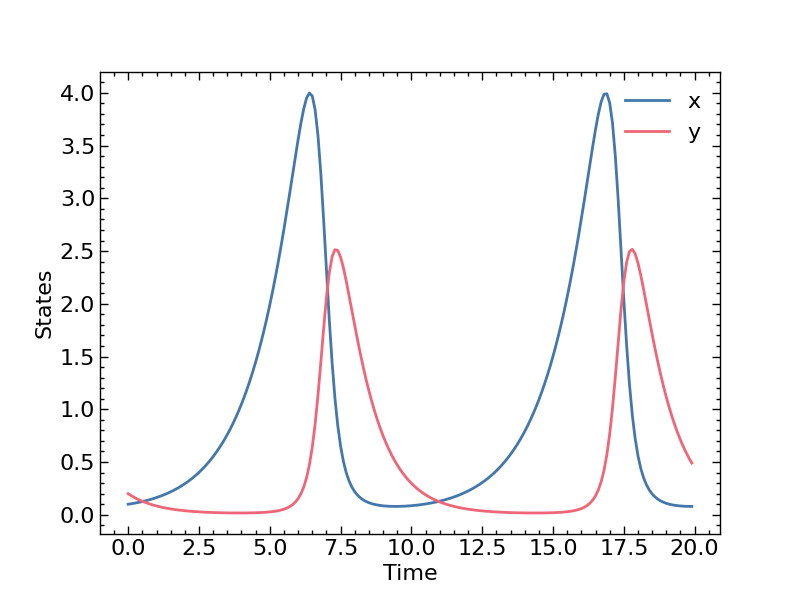
Note that this function is not yet differentiable, so we will need to define custom derivative rules. However, we can still test its correctness by simulating any differential equation. We will consider the classic Lotka-Volterra system

\[\begin{equation} \begin{aligned} \frac{dx}{dt} & = p_1 x + p_2 x y \\ \frac{dy}{dt} & = p_3 y + p_4 x y \end{aligned} \end{equation}\]

with parameters $p_1 = 2/3, \ p_2 = - 4/3, \ p_3 = - 1, \ p_4 = 1$, initial conditions $ x(t = 0) = 0.1, \ y(t = 0) = 0.2$, and time horizon as [$t_0 = 0, \ t_f = 20, \ \Delta t = 0.1$]. We will also use the classic LSODA method to integrate the Lotka-Volterra dynamics.

def LotkaVolterra(x, t, p) : 
    return jnp.array([
        p[0] * x[0] + p[1] * x[0] * x[1], 
        p[2] * x[1] + p[3] * x[0] * x[1]
    ])

t = jnp.arange(0, 20., 0.1)
x = jnp.array([0.1, 0.2])
p = jnp.array([2/3, -4/3, -1, 1])

solution = odeint(LotkaVolterra, x, t, p, method = "LSODA")

3. Defining Custom Reverse-Mode Automatic Differentiation Rule

In this section, we will derive the reverse-mode sensitivity (derivative) equations of ordinary differential equations and implement them in JAX. There are two approaches to computing sensitivities through a differential equation solver:

Discretize-then-Optimize : In this approach, the ODE solver first integrates the differential equation, producing a sequence of algebraic equations. These discrete equations are then differentiated to obtain the sensitivities. This method requires the ODE solver to be compatible with an automatic differentiation framework.
Optimize-then-Discretize : In this approach, the sensitivity equations are first derived in continuous/discrete form as differential equations. The resulting augmented system (comprising both the original dynamics and the sensitivity dynamics) is then integrated using any ODE solver. This method does not require the solver to be compatible with an automatic differentiation framework, allowing the use of any black-box solver.

In this tutorial, we will implement the Optimize-then-Discretize approach and derive the corresponding equations below. Consider the following dynamical equations

\[\begin{equation} \begin{aligned} & \hat{x}_0 = x_0 \\ & \frac{dx}{dt} = f(x, p), \quad t \in [0, N] \\ & \Phi = \phi(x_{N}) \end{aligned} \end{equation}\]

where $x$ and $f$ are the states and the dynamic equation. The parameters of the dynamic equations are $p$, $\Phi$ is the objective function. Note that the derivation can readily be extended to a more general case when the objective function depends on $x_1, \cdots, x_N$. However for brevity, we assume that the objective function only depends on $x_N$. The continuous-time dynamic equations can be converted to discrete-time system using an appropriate adaptive/fixed time-stepping method as follows

\[\begin{equation} \begin{aligned} & \hat{x}_0 = x_0 \\ & x_{k + 1} = F(x_k, p), \quad k = 0, ... \ N \\ & \Phi = \phi(x_{N}) \end{aligned} \end{equation}\]

To calculate the reverse-mode sensitivities we form the Lagrangian as follows

\[\begin{equation} L(\lambda, x_0, p) = \Phi + \lambda _0^T (\hat{x}_0 = x_0) + \sum _{k = 0} ^ {N - 1} \lambda _{k + 1}^{T} (F(x_k, p) - x_{k + 1}) \end{equation}\]

where $\lambda $ are the Lagrange multipliers, $x_0$ is the initial condition, and $p$ are the parameters. Taking the derivative of the Lagrangian with respect to $x_0$, and $p$ and equating to zero gives the sensitivity equations

\[\begin{equation} \begin{aligned} \frac{\partial{L}}{\partial x_0} & = \frac{d \Phi}{dx_N} \frac{\partial x_N}{\partial x_0} + \lambda _0^T + \sum _{k = 0}^{N - 1} \lambda _{k + 1}^{T} \left( \frac{\partial F(x_k, p)}{\partial x_k}\frac{\partial x_k}{\partial x_0} - \frac{\partial x_{k + 1}}{\partial x_0} \right) \\ \end{aligned} \end{equation}\] \[\begin{equation} \begin{aligned} \frac{\partial L}{\partial p } & = \sum _{k = 0}^{N - 1} \lambda _{k + 1}^{T} \left( \frac{\partial F(x_k, p)}{\partial p} \right) \end{aligned} \end{equation}\]

Differentiating the Lagrangian with respect to $\lambda$ gives back the dynamic Equations 3 and therefore the step is skipped. To find the derivative with respect to $p$, we need $\lambda _k$, which can be obtained from the above equation. Collecting all the $ \frac{dx_k}{dx_0} $ terms together gives

\[\begin{equation} \begin{aligned} \frac{\partial{L}}{\partial x_0} & = \left( \frac{d\Phi}{dx_N} - \lambda _N^T \right) \frac{\partial x_N}{\partial x_0} + \sum _{k = 0}^{N - 1} \left( - \lambda _{k}^T + \lambda _{k + 1}^T \frac{\partial F(x_k, p)}{\partial x_k} \right) \frac{\partial x_k}{\partial x_0} \end{aligned} \end{equation}\]

If we define $\lambda$ to be the solution of the system of equations mentioned below, then we can calculate $\frac{\partial L}{\partial p}$ by plugging the values of $\lambda _k$ in Equation 6.

\[\begin{equation} \begin{aligned} \lambda _N^T & = \frac{d\Phi}{dx_N} \\ \lambda _{k}^T & = \lambda _{k + 1}^T \frac{\partial F(x_k, p)}{\partial x_k}, \quad k = n - 1, \ldots \ 0 \end{aligned} \end{equation}\]

Equation 8 initializes the terminal value of $\lambda _N$, Equation 10 requires you to solve addition differential equations $\lambda ^T \frac{\partial F(x, p)}{\partial x} $ backward in time. We will now implement this in JAX using the jax.custom_vjp function to define custom reverse-mode derivatives for our _solve_ivp function. We will define a separate function, aug, which integrates the augmented dynamics, and another function, aug_jac, which computes the Jacobian of the augmented dynamics (required for implicit solvers). The augmented system is then integrated using our SciPy integrator, handled through the _solve_ivp_aug function.

@jax.custom_vjp
def _solve_ivp(x, t, p):
    result_shape = jax.ShapeDtypeStruct((len(t), x.shape[-1]), x.dtype)
    return jax.pure_callback(solve_ivp_host, result_shape, x, t, p) 

def aug(x, t, p):
    # Augmented system of differential equations
    x, ct_x, _ = jnp.array_split(x, [nx, 2 * nx])
    primals, vjp_func = jax.vjp(lambda _x, _p : afunc(_x, t, _p), x, p)
    return -jnp.concatenate([-primals, *vjp_func(ct_x)])

def aug_jac(t, x, p):
    # Jacobian of the augmented system is used by implicit methods of solve_ivp 
    return jax.jacrev(aug, argnums = 0)(x, t, p) 

def solve_ivp_aug_host(x, t, p):
    # If forward pass is evaluated then gradient should be calculated. 
    # Therefore there is no point in returning inf
    solution = solve_ivp(lambda _t, _x, _p : aug(_x, _t, _p), [t[0], t[-1]], x, t_eval = t, args = (p, ), 
                        rtol = rtol, atol = atol, jac = aug_jac, **kwargs)
    return solution.y.T

def _solve_ivp_aug(x, t, p):
    result_shape = jax.ShapeDtypeStruct((2, x.shape[-1]), x.dtype)
    return jax.pure_callback(solve_ivp_aug_host, result_shape, x, t, p) 

def _solve_ivp_fwd(x, t, p):
    # The function defining the forward pass of _solve_ivp
    solution = _solve_ivp(x, t, p)
    return solution, (x, t, p, solution)

def _solve_ivp_bwd(res, gdot):
    # The function defining the reverse pass of _solve_ivp
    x, t, p, solution = res

    def body_func(carry, state):
        xi, _gdot, t_start, t_end = state
        solution = _solve_ivp_aug(jnp.concatenate([xi, *carry]), jnp.array([t_start, t_end]), p)
        _, ct_x, ct_p = jnp.array_split(solution[-1], [nx, 2 * nx])
        return (ct_x + _gdot, ct_p), None  

    solution, _ = jax.lax.scan(body_func, (gdot[-1], jnp.zeros_like(p)), (solution[1:], gdot[:-1], t[1:], t[:-1]), reverse = True)
    return solution[0], None, solution[1]

_solve_ivp.defvjp(_solve_ivp_fwd, _solve_ivp_bwd)

And that’s it. We can now compare these gradients with gradients obtained using finite difference. To do so we form a simple objective function as follows

def obj(x, t, p):
    solution = odeint(LotkaVolterra, x, t, p, method = "LSODA")
    return jnp.mean((solution - jnp.ones_like(solution))**2)

loss, gradients = jax.value_and_grad(obj, argnums = (0, 1, 2))(x, t, p)


def fd(eps):
    vars, unravel = flatten_util.ravel_pytree((x, t, p))
    grads = jax.vmap(
        lambda v : (obj(*unravel(vars + eps * v)) - loss) / eps
    )(jnp.eye(len(vars)))
    return unravel(grads)

eps = 1e-4
fd_x, fd_t, fd_p = fd(eps)

Gradient (x) using automatic differentiation [-5.73076174 -1.23059696]
Gradient (x) using finite difference [-5.72760597 -1.23287042]
Gradient (p) using automatic differentiation [ 0.16888207  0.40636067 -1.92547423 -2.03613647]
Gradient (p) using finite difference [ 0.16914695  0.40360581 -1.92534344 -2.03573354]

This implementation now allows us to use any of the SciPy ODE solvers, with the added benefit of being fully reverse-mode differentiable.

4. Defining Custom Forward-Mode Automatic Differentiation Rule

Forward-mode sensitivity equations can be obtained by simply differentiating Equation 3 with respect to $x_0$ and $p$. We get the following equations

\[\begin{equation} \begin{aligned} & s_0 = I \\ & s_{k + 1} = \frac{\partial F(x_k, p)}{\partial x_k} s_k, \quad k = 0, \cdots ,\ N - 1, \quad s_k = \frac{\partial x_{k}}{\partial x_0} \\ & \frac{dx_{k + 1}}{dp} = \frac{\partial F(x_k, p)}{\partial x_k} \frac{\partial x_k}{\partial p} + \frac{\partial F(x_k, p)}{\partial p}, \quad k = 0, \cdots, \ N - 1 \\ & \frac{\partial \phi}{\partial x_0} = \frac{\partial \phi}{\partial x_{N}} s_N \end{aligned} \end{equation}\]

To implement this in JAX, we will now use the jax.custom_jvp function to define the custom forward-mode derivatives for our _solve_ivp function.

@jax.custom_jvp
def _solve_ivp(x, t, p):
    result_shape = jax.ShapeDtypeStruct((nt, x.shape[-1]), x.dtype)
    return jax.pure_callback(solve_ivp_host, result_shape, x, t, p) 

def aug(x, t, p):
    # Augmented system of differential equations
    p, p_tangent = jnp.array_split(p, 2)
    x, dx_dx0, dx_dp = jnp.array_split(x, 3)
    return jnp.concatenate([
        *jax.jvp(lambda x : afunc(x, t, p), (x, ), (dx_dx0, )),
        jax.jvp(lambda x, p : afunc(x, t, p), (x, p), (dx_dp, p_tangent))[-1]
    ])

def aug_jac(t, x, p):
    # Jacobian of the integrated function is used by implicit methods of solve_ivp 
    return jax.jafwd(aug, argnums = 0)(x, t, p) 

def solve_ivp_aug_host(x, t, p):
    # If forward pass is evaluated then gradient should be calculated. 
    # Therefore there is no point in returning inf
    solution = solve_ivp(lambda _t, _x, _p : aug(_x, _t, _p), [t[0], t[-1]], x, t_eval = t, args = (p, ), 
                        rtol = rtol, atol = atol, jac = aug_jac, **kwargs)
    return solution.y.T

def _solve_ivp_aug(x, t, p):
    result_shape = jax.ShapeDtypeStruct((nt, x.shape[-1]), x.dtype)
    return jax.pure_callback(solve_ivp_aug_host, result_shape, x, t, p) 

def _solve_ivp_fwd(primals, tangents):
    
    x, t, p = primals 
    xdot, _, p_dot = tangents 
    solution = _solve_ivp_aug(jnp.concatenate((x, xdot, jnp.zeros_like(xdot))), t, jnp.concatenate((p, p_dot)))
    solution, xtangent, ptangent = jnp.array_split(solution, 3, axis = 1)
    return solution, xtangent + ptangent

_solve_ivp.defjvp(_solve_ivp_fwd)

We again compare these gradients with gradients obtained using finite difference.

Gradient (x) using automatic differentiation [-5.73084119 -1.23060337]
Gradient (x) using finite difference [-5.72760597 -1.23287042]
Gradient (p) using automatic differentiation [ 0.16885783  0.4063586  -1.92548531 -2.03615103]
Gradient (p) using finite difference [ 0.16914695  0.40360581 -1.92534344 -2.03573354]

This cocludes our tutorial