Parameter estimation of ordinary differential equations using CasADi
Table of Contents
- Parameter Estimation
- CasADi
- Forward Simulation
- Single Shooting
- Multiple Shooting
- Orthogonal Collocation
- References
1. Parameter Estimation
Parameter estimation is a process of finding the optimal parameters of a given model using experimental data. In this tutorial, we will estimate the parameters of an ordinary differential equation (ODE) using three different methods
- Single shooting (Sequential optimization)
- Multiple shooting (Simultaneous optimization)
- Orthogonal Collocation (Simultaneous optimization)
We will implement these methods using CasADi
2. CasADi
CasADi is a open-source python package for automatic differentiation and nonlinear optimization 1. A lot of problems including parameter estimation of ODE’s can be efficiently solved using CasADi. In this section we will quicklly walk through the basic syntax of CasADi. We begin by importing required packages.
import numpy as np
import casadi as cd
import matplotlib.pyplot as plt
CasADi essentially creates symbolic expressions by treating everyting as matrix operation i.e vectors are treated as $n\times1$ matrix and scalar as $1\times1$ matrix. It has two basic data structures
-
The SX symbolics : used to define matrices where mathematical operations are performed element wise.
>>> x = cd.SX.sym("x", 2, 2) >>> 2 * x + 1 SX(@1=2, @2=1, [[((@1*x_0)+@2), ((@1*x_2)+@2)], [((@1*x_1)+@2), ((@1*x_3)+@2)]]) -
The MX symbolics : used to define matrices where mathematical operations are performed over the entire matrix.
  >>> x = cd.MX.sym("x", 2, 2)
  >>> 2 * x + 1
  MX((ones(2x2)+(2.*x)))
Once symbolic variables are defined, you can create mathematical expressions directly using CasADi primitives:
- Mathematical operations such as addition (
x + x), multiplication (x * x), trignometric functions (cd.sin(x)), matrix multiplications (cd.mtimes(x, x)) - Linear algebra such as solving linear systems (
cd.solve(A, b)), root finding problem (cd.rootfinder(g)) - Control flow such as if-else statements (
cd.if_else(*args)) - Automatic differentiation using forward (Jacobian-vector-product) and reverse mode (vector-Jacobian-product) (
cd.jacobian(A@x, x))
Using these mathematical expressions, CasADi can also be used for optimization. Lets look at the CasADi syntax for solving a simple optimization problem given below using the cd.Opti optimization helper class
opti = cd.Opti() # Initialize CasADi optimization helper class
p = opti.variable(2) # Define decision variables

opti.minimize((p[0] - 1)**2 + (p[1] - 2)**2) # Define objective function
opti.subject_to(p[0] >= 2) # Define constraints
opti.set_initial(p, np.array([0, 0])) # Define initial conditions

plugin_options = {} # Plugin options
solver_options = {"max_iter" : 100, "tol" : 1e-5} # solver options
opti.solver("ipopt", plugin_options, solver_options) # Initialize optimization solver
optimal = opti.solve() # Solve the problem
print("Optimal Parameters : ", optimal.value(p)) # Get the optimal parameters
This is Ipopt version 3.12.3, running with linear solver mumps.
NOTE: Other linear solvers might be more efficient (see Ipopt documentation).

Number of nonzeros in equality constraint Jacobian...:        0
Number of nonzeros in inequality constraint Jacobian.:        1
Number of nonzeros in Lagrangian Hessian.............:        2

Total number of variables............................:        2
                     variables with only lower bounds:        0
                variables with lower and upper bounds:        0
                     variables with only upper bounds:        0
Total number of equality constraints.................:        0
Total number of inequality constraints...............:        1
        inequality constraints with only lower bounds:        1
   inequality constraints with lower and upper bounds:        0
        inequality constraints with only upper bounds:        0

iter    objective    inf_pr   inf_du lg(mu)  ||d||  lg(rg) alpha_du alpha_pr  ls
   0  5.0000000e+00 2.00e+00 4.00e+00  -1.0 0.00e+00    -  0.00e+00 0.00e+00   0
   1  1.1597632e+00 0.00e+00 1.00e-06  -1.0 2.08e+00    -  1.00e+00 1.00e+00f  1
   2  1.0127481e+00 0.00e+00 2.83e-08  -2.5 7.06e-02    -  1.00e+00 1.00e+00f  1
   3  1.0002282e+00 0.00e+00 1.50e-09  -3.8 6.24e-03    -  1.00e+00 1.00e+00f  1
   4  1.0000018e+00 0.00e+00 1.84e-11  -5.7 1.13e-04    -  1.00e+00 1.00e+00f  1

Number of Iterations....: 4

                                   (scaled)                 (unscaled)
Objective...............:   1.0000018305414848e+00    1.0000018305414848e+00
Dual infeasibility......:   1.8449242134011001e-11    1.8449242134011001e-11
Constraint violation....:   0.0000000000000000e+00    0.0000000000000000e+00
Complementarity.........:   1.8705423593317057e-06    1.8705423593317057e-06
Overall NLP error.......:   1.8705423593317057e-06    1.8705423593317057e-06


Number of objective function evaluations             = 5
Number of objective gradient evaluations             = 5
Number of equality constraint evaluations            = 0
Number of inequality constraint evaluations          = 5
Number of equality constraint Jacobian evaluations   = 0
Number of inequality constraint Jacobian evaluations = 5
Number of Lagrangian Hessian evaluations             = 4
Total CPU secs in IPOPT (w/o function evaluations)   =      0.002
Total CPU secs in NLP function evaluations           =      0.000

EXIT: Optimal Solution Found.
      solver  :   t_proc      (avg)   t_wall      (avg)    n_eval
       nlp_f  |  18.00us (  3.60us)  18.96us (  3.79us)         5
       nlp_g  |  15.00us (  3.00us)  16.18us (  3.24us)         5
  nlp_grad_f  |  27.00us (  4.50us)  26.11us (  4.35us)         6
  nlp_hess_l  |  14.00us (  3.50us)  15.03us (  3.76us)         4
   nlp_jac_g  |  16.00us (  2.67us)  17.27us (  2.88us)         6
       total  |   2.71ms (  2.71ms)   2.72ms (  2.72ms)         1
--------------------------------------------------------------------------------
Optimal Parameters :  [2.00000092 2.        ]
3. Forward Simulation
Now we will look at how to forward simulate and ordinary differential equation in CasADi. We will use the classic Lotka-Volterra system with the following dynamics
\[\begin{equation} \begin{aligned} \frac{dx}{dt} & = p_1 x + p_2 x y \\ \frac{dy}{dt} & = p_3 y + p_4 x y \end{aligned} \end{equation}\]with parameters $p_1 = 2/3, \ p_2 = - 4/3, \ p_3 = - 1, \ p_4 = 1$, initial conditions $ x(t = 0) = 0.1, \ y(t = 0) = 0.2$, and time horizon as [$t_0 = 0, \ t_f = 20, \ \Delta t = 0.1$].
# Define the dynamic equation
def LotkaVolterra(x, t, p):
    return cd.vertcat(
        p[0] * x[0] + p[1] * x[0] * x[1],
        p[2] * x[1] + p[3] * x[0] * x[1]
    )

x = cd.MX.sym("x", 2) # CasADi symbolic for states
p = cd.MX.sym("p", 4) # CasADi symbolic for parameters

# Define ODE dictionary
ode = {
    "x" : x, # States
    "p" : p, # Parameters
    "ode" : LotkaVolterra(x, 0, p), # Dynamic equation
}

dt = 0.1 # time interval
t0, tf = 0, 20 # Initial and Final time
xinit = np.array([1, 2]) # Initial conditions
parameters = np.array([2/3, -4/3, -1, 1]) # Parameters
time_span = np.arange(t0, tf, dt) # Time span


# Define CasADi integrator object
F = cd.integrator(
    "F", # Name
    "cvodes", # ODE solver
    ode, # ODE dictionary
    {"t0" : t0, "tf" : dt}
)

F_map = F.mapaccum(len(time_span) - 1) # Forward simulate N times
solution = F_map(x0 = xinit, p = parameters)["xf"].toarray().T # Get the solution
solution = np.row_stack((xinit, solution))

# Plotting the solution
with plt.style.context(["science", "notebook", "bright"]):

    plt.plot(time_span, solution, label = ["x", "y"])
    plt.xlabel("Time")
    plt.ylabel("States")
    plt.legend()
    plt.show()
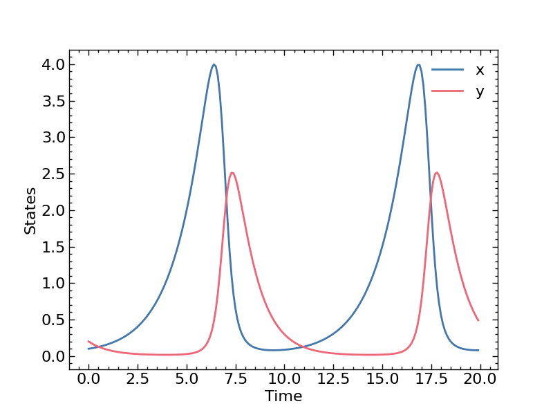
Now that we have generated synthetic data, the following sections will explore different methods for estimating the true parameters from this data.
4. Single Shooting
Probably the most straightforward method is called single-shooting 2. In this approach, you solve the optimization problem given below. For a given set of parameter values at any iteration, an ODE solver is used to compute the state trajectory, which is then used to evaluate the loss. The parameter values are then updated using gradients computed through the ODE solver. Note that in this tutorial, I will not go into the details of how derivatives are computed across the ODE solver. However, it is worth mentioning that in CasADi, using rk computes derivatives via the discretize-then-optimize approach, while cvodes computes them using the optimize-then-discretize method 3.
If we take a simple examples 4, as shown in the below figure, you fire the cannon, check if the ball landed at the desired target point, adjust your velocity and repeat.

In this case, we need to pass the decision variables, defined using the cd.Opti helper class, into the cd.integrator class to obtain the state trajectories. These states are then used to compute the objective function that needs to be minimized. Let’s look at the code:
parameters = opti.variable(4) # Define decision variables
trajectory = F_map(x0 = xinit, p = parameters)["xf"].T # Instead of the original parameter, pass the decision variables
opti.minimize(cd.sumsqr(solution[1:] - trajectory)) # Minimize sum of squared error
opti.set_initial(parameters, np.array([1, -1, -1, 1])) # Set initial conditions of parameters

opti.solver("ipopt", plugin_options, solver_options)
optimal = opti.solve()
And that’s all !
This is Ipopt version 3.12.3, running with linear solver mumps.
NOTE: Other linear solvers might be more efficient (see Ipopt documentation).

Number of nonzeros in equality constraint Jacobian...:        0
Number of nonzeros in inequality constraint Jacobian.:        0
Number of nonzeros in Lagrangian Hessian.............:       10

Total number of variables............................:        4
                     variables with only lower bounds:        0
                variables with lower and upper bounds:        0
                     variables with only upper bounds:        0
Total number of equality constraints.................:        0
Total number of inequality constraints...............:        0
        inequality constraints with only lower bounds:        0
   inequality constraints with lower and upper bounds:        0
        inequality constraints with only upper bounds:        0

iter    objective    inf_pr   inf_du lg(mu)  ||d||  lg(rg) alpha_du alpha_pr  ls
   0  1.3237413e+03 0.00e+00 1.00e+02  -1.0 0.00e+00    -  0.00e+00 0.00e+00   0
   1  1.2885654e+03 0.00e+00 1.02e+02  -1.0 1.01e-02   4.0 1.00e+00 1.00e+00f  1
   2  1.1837822e+03 0.00e+00 1.10e+02  -1.0 3.25e-02   3.5 1.00e+00 1.00e+00f  1
   3  6.2565374e+02 0.00e+00 2.45e+02  -1.0 1.56e-01   3.0 1.00e+00 1.00e+00f  1
   4  2.1087328e+02 0.00e+00 2.83e+02  -1.0 1.71e-01   3.5 1.00e+00 1.00e+00f  1
   5  2.0954055e+02 0.00e+00 3.31e+02  -1.0 1.88e-01   3.0 1.00e+00 5.00e-01f  2
   6  4.4672675e+01 0.00e+00 1.33e+02  -1.0 2.81e-01   2.5 1.00e+00 2.50e-01f  3
   7  5.8595194e+00 0.00e+00 1.63e+01  -1.0 1.29e-01    -  1.00e+00 1.00e+00f  1
   8  4.3107360e-01 0.00e+00 4.08e+00  -1.0 1.05e-01    -  1.00e+00 1.00e+00f  1
   9  8.2359546e-03 0.00e+00 7.11e-01  -1.0 4.92e-02    -  1.00e+00 1.00e+00f  1
iter    objective    inf_pr   inf_du lg(mu)  ||d||  lg(rg) alpha_du alpha_pr  ls
  10  6.1401598e-06 0.00e+00 3.07e-02  -1.7 8.34e-03    -  1.00e+00 1.00e+00f  1
  11  7.3325122e-11 0.00e+00 3.11e-05  -2.5 2.19e-04    -  1.00e+00 1.00e+00f  1
  12  2.1898137e-15 0.00e+00 6.56e-07  -5.7 5.10e-07    -  1.00e+00 1.00e+00f  1

Number of Iterations....: 12

                                   (scaled)                 (unscaled)
Objective...............:   1.1654087765916845e-16    2.1898137210350870e-15
Dual infeasibility......:   6.5611246857218809e-07    1.2328413129198253e-05
Constraint violation....:   0.0000000000000000e+00    0.0000000000000000e+00
Complementarity.........:   0.0000000000000000e+00    0.0000000000000000e+00
Overall NLP error.......:   6.5611246857218809e-07    1.2328413129198253e-05


Number of objective function evaluations             = 24
Number of objective gradient evaluations             = 13
Number of equality constraint evaluations            = 0
Number of inequality constraint evaluations          = 0
Number of equality constraint Jacobian evaluations   = 0
Number of inequality constraint Jacobian evaluations = 0
Number of Lagrangian Hessian evaluations             = 12
Total CPU secs in IPOPT (w/o function evaluations)   =      0.112
Total CPU secs in NLP function evaluations           =     10.938

EXIT: Optimal Solution Found.
      solver  :   t_proc      (avg)   t_wall      (avg)    n_eval
       nlp_f  | 628.84ms ( 26.20ms) 630.20ms ( 26.26ms)        24
  nlp_grad_f  |   2.21 s (157.99ms)   2.22 s (158.27ms)        14
  nlp_hess_l  |  12.90 s (  1.08 s)  12.93 s (  1.08 s)        12
       total  |  15.75 s ( 15.75 s)  15.78 s ( 15.78 s)         1
--------------------------------------------------------------------------------
Optimal Parameters :  [ 0.66666667 -1.33333333 -1.          1.        ]
5. Multiple Shooting
In single-shooting, the parameters are the only decision variables in the optimization problem, while the states are obtained by integrating the dynamic equations using the current parameter estimates. However, if the model is oscillatory or if the parameters take on “bad” values, integrating over long trajectories can become computationally expensive or even unstable. To overcome these issues, multiple-shooting is often used. This method divides the long trajectory into shorter intervals that can be integrated in parallel, while enforcing continuity conditions between intervals. As a consequence, the optimization problem grows in dimension, since the initial states of each interval must now also be treated as decision variables. Nevertheless, at each iteration of the optimization procedure, a sparse system of equations is solved, and CasADi exploits this sparsity to improve efficiency.
An equivalent example is shown in the figure below. For comparison, the corresponding multiple-shooting optimization problem with only two intervals is also illustrated.

Fortunately, the code does not change a lot. We just have to define the initial states of the intervals as additinal decision variables.
intervals = 2 # Define the number of intervals
x = opti.variable(2, intervals) # Define initial states at each intervals as decision variables
parameters = opti.variable(4) # Define decision variables
F_map = F.mapaccum(len(time_span) // intervals) # Account for small integration spans

trajectory = []
xi = xinit
for i in range(intervals) :
    traj = F_map(x0 = xi, p = parameters)["xf"] # Get the solution
    xi = x[:, i]
    opti.subject_to(traj[:, -1] - xi == 0) # continuite constraints
    trajectory.append(traj.T) # stack solution

opti.minimize(cd.sumsqr(solution[1:] - cd.vertcat(*trajectory)[:-1, :])) # Minimize sum of squared error
opti.set_initial(parameters, np.array([1, -1, -1, 1])) # Set initial conditions of parameters
opti.set_initial(x, 0.1) # set initial conditions of states

plugin_options = {}
solver_options = {"max_iter" : 100, "tol" : 1e-5}
opti.solver("ipopt", plugin_options, solver_options)
optimal = opti.solve()
print("Optimal Parameters : ", optimal.value(parameters))
This is Ipopt version 3.12.3, running with linear solver mumps.
NOTE: Other linear solvers might be more efficient (see Ipopt documentation).

Number of nonzeros in equality constraint Jacobian...:       24
Number of nonzeros in inequality constraint Jacobian.:        0
Number of nonzeros in Lagrangian Hessian.............:       21

Total number of variables............................:        8
                     variables with only lower bounds:        0
                variables with lower and upper bounds:        0
                     variables with only upper bounds:        0
Total number of equality constraints.................:        4
Total number of inequality constraints...............:        0
        inequality constraints with only lower bounds:        0
   inequality constraints with lower and upper bounds:        0
        inequality constraints with only upper bounds:        0

iter    objective    inf_pr   inf_du lg(mu)  ||d||  lg(rg) alpha_du alpha_pr  ls
   0  1.3385487e+03 1.97e-01 7.43e+01  -1.0 0.00e+00    -  0.00e+00 0.00e+00   0
   1  1.0810006e+03 5.25e-02 4.99e+02  -1.0 9.49e-02   4.0 1.00e+00 1.00e+00f  1
   2  8.4946624e+02 9.31e-03 1.97e+02  -1.0 5.92e-02   3.5 1.00e+00 1.00e+00f  1
   3  6.0997460e+02 8.10e-03 1.74e+02  -1.0 5.91e-02   3.0 1.00e+00 1.00e+00f  1
   4  5.0374473e+02 2.84e-03 7.62e+01  -1.0 2.57e-02   3.5 1.00e+00 1.00e+00f  1
   5  1.8674163e+02 3.76e-02 6.39e+01  -1.0 6.47e-02   3.0 1.00e+00 1.00e+00f  1
   6  3.0464485e+01 9.24e-02 1.09e+02  -1.0 1.39e-01    -  1.00e+00 1.00e+00f  1
   7  2.0692181e+00 9.50e-03 1.73e+01  -1.0 7.55e-02    -  1.00e+00 1.00e+00f  1
   8  7.7028395e-02 1.97e-03 2.28e+00  -1.0 5.88e-02    -  1.00e+00 1.00e+00f  1
   9  3.1099600e-04 1.95e-04 1.72e-01  -1.0 2.04e-02    -  1.00e+00 1.00e+00h  1
iter    objective    inf_pr   inf_du lg(mu)  ||d||  lg(rg) alpha_du alpha_pr  ls
  10  5.8960977e-09 8.13e-07 6.84e-04  -2.5 1.40e-03    -  1.00e+00 1.00e+00h  1
  11  1.5567896e-15 6.46e-11 7.23e-07  -5.7 5.38e-06    -  1.00e+00 1.00e+00h  1

Number of Iterations....: 11

                                   (scaled)                 (unscaled)
Objective...............:   7.3046282179639731e-17    1.5567895805068316e-15
Dual infeasibility......:   7.2261163101897737e-07    1.5400568302118884e-05
Constraint violation....:   6.4577357350437126e-11    6.4577357350437126e-11
Complementarity.........:   0.0000000000000000e+00    0.0000000000000000e+00
Overall NLP error.......:   7.2261163101897737e-07    1.5400568302118884e-05


Number of objective function evaluations             = 12
Number of objective gradient evaluations             = 12
Number of equality constraint evaluations            = 12
Number of inequality constraint evaluations          = 0
Number of equality constraint Jacobian evaluations   = 12
Number of inequality constraint Jacobian evaluations = 0
Number of Lagrangian Hessian evaluations             = 11
Total CPU secs in IPOPT (w/o function evaluations)   =      0.253
Total CPU secs in NLP function evaluations           =     11.914

EXIT: Optimal Solution Found.
      solver  :   t_proc      (avg)   t_wall      (avg)    n_eval
       nlp_f  | 315.51ms ( 26.29ms) 316.05ms ( 26.34ms)        12
       nlp_g  | 316.31ms ( 26.36ms) 316.97ms ( 26.41ms)        12
  nlp_grad_f  |   1.88 s (144.91ms)   1.89 s (145.17ms)        13
  nlp_hess_l  |  11.87 s (  1.08 s)  11.89 s (  1.08 s)        11
   nlp_jac_g  |   2.30 s (176.69ms)   2.30 s (176.99ms)        13
       total  |  16.68 s ( 16.68 s)  16.71 s ( 16.71 s)         1
--------------------------------------------------------------------------------
Optimal Parameters :  [ 0.66666667 -1.33333333 -1.          1.        ]
6. Orthogonal Collocation
In both single- and multiple-shooting an ODE integrator and as subroutine to compute the derivatives across this integrator is required. Computing these derivatives is usually the most expensive step in these shooting methods. Collocation based methods approximates the solution of the states using a polynomial and therefore curcumvents the need for an ODE integrator and its subroutine 5. Specifically, orthogonal collocation uses Lagrange interpolation polynomial given as
\[\begin{equation} \begin{aligned} & x_i^K(t) = \sum_{j = 0}^{K} L_j(\tau)x_{i, j} \\ \text{where} \quad & L_j(\tau) = \prod _{k = 0, \ k \neq j}^K \frac{(\tau - \tau_k)}{(\tau_j - \tau_k)}, \quad \tau = \frac{t - t_i}{t_{i + 1} - t_i} \end{aligned} \end{equation}\]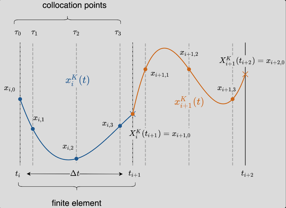
where $K$ is the degree of the polynomial with $K + 1$ collocation points, $\tau \in [0, 1]$ is a dimensionless time, $L_j(\tau)$ is the Lagrange basis polynomial such that $L_j(\tau_j) = 1$ and $L_j(\tau_i) = 0$ for all other interpolation points $i \neq j$. The variable $x_i^K$ is the value of the state at the $i$-th interval and the $K$-th collocation point. These values, together with the parameters, are unknown and form the decision variables of the problem.
-
Dynamic/Collocation Constraints
Once you have the interpolating polynomial for the states, the dynamic equation can be used to incorporate constriants. Specifically, the time derivatives from the polynomial approximation evaluated at the collocation points must be equal to the dynamic equation at the same points.
\[\begin{equation} \begin{aligned} \frac{dx_i^K}{dt} \Bigg|_{t_{i, k}} & = f(x_{i, k}, p), \quad \forall \ k \in [1, \cdots, K] \\ \text{where} \quad \frac{dx_i^K}{dt} \Bigg|_{t_{i, k}} & = \sum _{j = 0}^K \frac{x_{i, j}}{t_{i + 1} - t_i}\underbrace{\frac{dL_j}{d\tau}}_{\text{precomputed}} \end{aligned} \end{equation}\] -
Continuity Constraints
Additional constraints are incorporated to ensure conitnuity between the finite elements. Just as we did in multiple-shooting, this can be achieved by simply enforcing equality constraints between the initial state of an interval and the final evaluated state from the previous interval.
\[\begin{equation} \begin{aligned} x_{i + 1, 0} = \sum _{j = 0}^K L_j(\tau = 1)x_{i, j} \end{aligned} \end{equation}\]
To summarize, we transformed the original optimization problem involving an integral into one with only algebraic objectives, equality constraints, and inequality constraints. However, this comes at the cost of increasing the number of decision variables: in addition to the parameters, the states at each collocation point must also be optimized. For long trajectories, higher-degree collocation polynomials, multiple initial conditions, or high-dimensional state spaces, solving such a problem directly becomes infeasible without exploiting sparsity. Fortunately, CasADi manages this automatically behind the scenes, making the overall optimization problem tractable.
The code is as follows
d = 3 # The degree of interpolating polynomial
tau_root = np.append(0, cd.collocation_points(d, "legendre")) # Get collocation points
B, C, D = get_collocation_coefficients(d) # Get the collocation coefficients. Computed offline

nx = 2 # Dimension of states
x_sym = cd.MX.sym("x", nx)
p_sym = cd.MX.sym("p", 4)

N = len(time_span) - 1 # Number of intervals
f = cd.Function('f', [x_sym, p_sym], [dt * LotkaVolterra(x_sym, 0, p_sym)], ['x', 'p'], ['xdot']) # Continuous time dynamics

parameters = opti.variable(4) # Parameters as decision variables
x_var = opti.variable(nx, N * (d + 1)) # Collocation states as decision variables
xk_end = cd.MX(xinit) # Given initial conditions
cost = 0 # Objective function

for k in range(N):

    xk = x_var[:, k * (d + 1) : (k + 1) * (d + 1)] # States at collocation points
    opti.subject_to(cd.vec(xk[:, 0] - xk_end) == 0) # Continuity constraints ad end points
    xp = cd.mtimes(xk, cd.MX(C[:, 1:])) # Expression for the state derivative at the collocation point

    opti.subject_to(cd.vec(f(xk[:, 1:], parameters) - xp) == 0) # Dynamic equation constraint at the collocation point
    xk_end = cd.mtimes(xk, cd.MX(D)) # Expression for the end state
    cost += cd.sumsqr(xk[:, 0] - solution[k]) # add objective function

opti.minimize(cost)
opti.set_initial(p_var, 0) # Initial conditions of parameters
opti.set_initial(x_var, 0.1) # Initial conditions of states

plugin_options = {}
solver_options = {"max_iter" : 100, "tol" : 1e-5}
opti.solver("ipopt", plugin_options, solver_options)
optimal = opti.solve()
print("Optimal Parameters : ", optimal.value(parameters))
This is Ipopt version 3.12.3, running with linear solver mumps.
NOTE: Other linear solvers might be more efficient (see Ipopt documentation).

Number of nonzeros in equality constraint Jacobian...:     6362
Number of nonzeros in inequality constraint Jacobian.:        0
Number of nonzeros in Lagrangian Hessian.............:     3184

Total number of variables............................:     1198
                     variables with only lower bounds:        0
                variables with lower and upper bounds:        0
                     variables with only upper bounds:        0
Total number of equality constraints.................:     1194
Total number of inequality constraints...............:        0
        inequality constraints with only lower bounds:        0
   inequality constraints with lower and upper bounds:        0
        inequality constraints with only upper bounds:        0

iter    objective    inf_pr   inf_du lg(mu)  ||d||  lg(rg) alpha_du alpha_pr  ls
   0  6.0324811e+02 1.00e-01 1.03e+00  -1.0 0.00e+00    -  0.00e+00 0.00e+00   0
   1  4.8656986e+02 2.07e-01 9.86e+01  -1.0 6.92e+00   0.0 1.00e+00 1.00e+00f  1
   2  4.0985418e+02 3.90e-01 3.00e+02  -1.0 5.40e+00   1.3 1.00e+00 1.00e+00f  1
   3  3.0930303e+02 3.02e-01 5.02e+03  -1.0 7.18e+00   0.9 1.00e+00 2.50e-01f  3
   4  3.7381705e+02 9.78e-02 1.49e+03  -1.0 2.17e+00    -  1.00e+00 1.00e+00h  1
   5  4.7153805e+02 8.35e-02 7.15e+02  -1.0 1.60e+00    -  1.00e+00 1.00e+00h  1
   6  5.2707499e+02 5.80e-02 1.45e+03  -1.0 9.27e-01   1.3 1.00e+00 1.00e+00h  1
   7  5.9992875e+02 3.13e-02 5.71e+04  -1.0 2.01e+00   2.6 1.00e+00 1.00e+00h  1
   8  5.8092412e+02 2.16e-03 5.71e+03  -1.0 3.25e-01   3.9 1.00e+00 1.00e+00f  1
   9  5.8247744e+02 1.29e-03 8.40e+03  -1.0 6.14e-01   3.5 1.00e+00 5.00e-01h  2
iter    objective    inf_pr   inf_du lg(mu)  ||d||  lg(rg) alpha_du alpha_pr  ls
  10  5.9109967e+02 3.00e-03 3.71e+03  -1.0 2.11e-01   3.0 1.00e+00 1.00e+00h  1
  11  6.0188048e+02 3.95e-03 3.23e+03  -1.0 3.97e-01   2.5 1.00e+00 1.00e+00H  1
  12  6.0395001e+02 3.28e-03 2.58e+03  -1.0 3.54e-01   2.9 1.00e+00 5.00e-01h  2
  13  6.0541438e+02 3.55e-03 9.95e+04  -1.0 2.73e-01   2.5 1.00e+00 1.00e+00H  1
  14  6.0595458e+02 4.03e-04 1.56e+04  -1.0 4.90e-02   2.0 1.00e+00 1.00e+00h  1
  15  6.0427039e+02 1.29e-03 6.47e+03  -1.0 7.65e-02   1.5 1.00e+00 1.00e+00f  1
  16  5.8868277e+02 5.14e-03 1.44e+03  -1.0 1.74e-01   1.0 1.00e+00 1.00e+00F  1
  17  5.8282079e+02 3.02e-03 2.02e+01  -1.0 1.07e-01   1.4 1.00e+00 1.00e+00f  1
  18  5.6532432e+02 2.02e-02 1.78e+02  -1.7 3.19e-01   1.0 1.00e+00 1.00e+00f  1
  19  5.0727059e+02 3.96e-01 1.61e+03  -1.7 1.04e+00   0.5 1.00e+00 1.00e+00f  1
iter    objective    inf_pr   inf_du lg(mu)  ||d||  lg(rg) alpha_du alpha_pr  ls
  20  5.2618730e+02 8.65e-02 3.29e+03  -1.7 4.28e-01   1.8 1.00e+00 1.00e+00h  1
  21  5.1572823e+02 8.12e-03 1.31e+02  -1.7 3.63e-01   1.3 1.00e+00 1.00e+00f  1
  22  5.1493541e+02 2.48e-03 4.35e+03  -1.7 1.80e-01   0.9 1.00e+00 1.00e+00f  1
  23  5.0190968e+02 2.39e-02 5.96e+02  -1.7 4.05e-01   0.4 1.00e+00 1.00e+00f  1
  24  4.9787933e+02 1.87e-03 9.85e+01  -1.7 1.46e-01   0.8 1.00e+00 1.00e+00f  1
  25  4.8983845e+02 1.93e-02 1.68e+02  -1.7 3.64e-01   0.3 1.00e+00 1.00e+00f  1
  26  4.8227748e+02 3.80e-01 8.09e+03  -1.7 2.69e+00  -0.1 1.00e+00 1.00e+00f  1
  27  4.8961614e+02 6.05e-02 4.26e+03  -1.7 1.61e+00   2.1 1.00e+00 1.00e+00h  1
  28  4.8848951e+02 3.47e-02 3.93e+03  -1.7 3.70e-01   1.6 1.00e+00 1.00e+00f  1
  29  4.7377523e+02 1.14e-02 5.30e+04  -1.7 3.69e-01   2.0 1.00e+00 1.00e+00f  1
iter    objective    inf_pr   inf_du lg(mu)  ||d||  lg(rg) alpha_du alpha_pr  ls
  30  4.7069980e+02 2.59e-02 4.50e+04  -1.7 3.56e-01   1.6 1.00e+00 1.00e+00f  1
  31  4.7350997e+02 9.42e-04 7.75e+03  -1.7 1.18e-01   2.0 1.00e+00 1.00e+00h  1
  32  4.7320275e+02 3.65e-05 8.04e+01  -1.7 2.00e-02   1.5 1.00e+00 1.00e+00f  1
  33  4.7266573e+02 2.25e-04 6.05e+00  -1.7 5.61e-02   1.0 1.00e+00 1.00e+00f  1
  34  4.7114766e+02 2.09e-03 2.26e+01  -2.5 1.69e-01   0.6 1.00e+00 1.00e+00f  1
  35  4.6732770e+02 1.96e-02 1.59e+02  -2.5 5.55e-01   0.1 1.00e+00 1.00e+00f  1
  36  4.6437372e+02 3.74e-03 2.77e+00  -2.5 2.32e-01   0.5 1.00e+00 1.00e+00f  1
  37  4.6006562e+02 2.30e-02 8.44e+01  -2.5 5.66e-01   0.0 1.00e+00 1.00e+00f  1
  38  4.5626620e+02 5.05e-03 2.62e+00  -2.5 2.83e-01   0.5 1.00e+00 1.00e+00f  1
  39  4.5092091e+02 3.23e-02 5.36e+01  -2.5 6.22e-01  -0.0 1.00e+00 1.00e+00f  1
iter    objective    inf_pr   inf_du lg(mu)  ||d||  lg(rg) alpha_du alpha_pr  ls
  40  4.4518753e+02 8.02e-03 5.52e+00  -2.5 3.96e-01   0.4 1.00e+00 1.00e+00f  1
  41  4.3814748e+02 5.42e-02 7.51e+01  -2.5 7.28e-01  -0.1 1.00e+00 1.00e+00f  1
  42  4.3193675e+02 1.58e-01 1.90e+02  -2.5 3.04e+00   0.4 1.00e+00 1.00e+00f  1
  43  4.2885993e+02 1.80e-02 1.36e+01  -2.5 1.07e+00   0.8 1.00e+00 1.00e+00f  1
  44  4.1487792e+02 3.23e-01 1.48e+02  -2.5 1.47e+00    -  1.00e+00 1.00e+00f  1
  45  4.0149536e+02 2.51e-02 1.03e+02  -2.5 4.18e-01   1.2 1.00e+00 1.00e+00f  1
  46  3.9371975e+02 3.93e-02 1.34e+02  -2.5 9.60e-01    -  1.00e+00 1.00e+00f  1
  47  3.8087831e+02 8.16e-03 1.24e+02  -2.5 2.68e-01   0.7 1.00e+00 1.00e+00f  1
  48  3.7557661e+02 6.48e-04 8.79e+00  -2.5 8.73e-02   1.2 1.00e+00 1.00e+00f  1
  49  3.6588265e+02 4.54e-03 3.05e+00  -2.5 2.39e-01   0.7 1.00e+00 1.00e+00f  1
iter    objective    inf_pr   inf_du lg(mu)  ||d||  lg(rg) alpha_du alpha_pr  ls
  50  3.3148883e+02 8.57e-02 1.20e+02  -2.5 1.11e+00   0.2 1.00e+00 1.00e+00f  1
  51  2.8891407e+02 3.02e-02 5.50e+01  -2.5 6.13e-01   0.6 1.00e+00 1.00e+00f  1
  52  2.2237976e+02 1.22e-01 5.81e+01  -2.5 1.47e+00   0.2 1.00e+00 1.00e+00f  1
  53  1.6796586e+02 2.91e-02 8.86e+01  -2.5 6.18e-01   0.6 1.00e+00 1.00e+00f  1
  54  1.0171260e+02 5.06e-02 6.81e+01  -2.5 1.12e+00   0.1 1.00e+00 1.00e+00f  1
  55  5.6179636e+01 5.05e-01 6.03e+02  -2.5 6.59e+00  -0.4 1.00e+00 5.00e-01f  2
  56  3.4328597e+01 3.74e-01 3.48e+02  -2.5 3.19e+00   0.1 1.00e+00 2.50e-01f  3
  57  4.8101692e+01 1.64e-01 7.27e+02  -2.5 1.70e+00   0.5 1.00e+00 1.00e+00h  1
  58  4.3005374e+01 1.67e-01 5.23e+02  -2.5 3.45e+00   0.9 1.00e+00 2.50e-01f  3
  59  3.9935621e+01 2.68e-01 1.28e+03  -2.5 3.30e+00   0.4 1.00e+00 5.00e-01f  2
iter    objective    inf_pr   inf_du lg(mu)  ||d||  lg(rg) alpha_du alpha_pr  ls
  60  3.0823055e+01 1.42e-02 3.07e+02  -2.5 3.82e-01   1.8 1.00e+00 1.00e+00f  1
  61  3.3862690e+01 1.25e-02 2.85e+02  -2.5 1.55e+00    -  1.00e+00 1.25e-01h  4
  62  3.6997095e+01 1.10e-02 2.62e+02  -2.5 1.55e+00    -  1.00e+00 1.25e-01h  4
  63  4.0034458e+01 9.64e-03 2.40e+02  -2.5 1.54e+00    -  1.00e+00 1.25e-01h  4
  64  4.2859075e+01 1.06e-02 2.17e+02  -2.5 1.49e+00    -  1.00e+00 1.25e-01h  4
  65  4.5378554e+01 1.20e-02 1.95e+02  -2.5 1.40e+00    -  1.00e+00 1.25e-01h  4
  66  4.7464915e+01 1.26e-02 1.74e+02  -2.5 1.25e+00    -  1.00e+00 1.25e-01h  4
  67  4.8902884e+01 1.23e-02 1.54e+02  -2.5 1.04e+00    -  1.00e+00 1.25e-01h  4
  68  4.8171647e+01 6.89e-03 1.44e+02  -2.5 7.75e-01    -  1.00e+00 1.00e+00H  1
  69  2.5687522e+01 5.85e-02 6.24e+02  -2.5 6.77e-01    -  1.00e+00 1.00e+00f  1
iter    objective    inf_pr   inf_du lg(mu)  ||d||  lg(rg) alpha_du alpha_pr  ls
  70  1.8365185e+01 6.37e-01 2.31e+03  -2.5 2.74e+00    -  1.00e+00 1.00e+00f  1
  71  1.0001658e+01 9.92e-02 8.53e+02  -2.5 1.12e+00   1.3 1.00e+00 1.00e+00f  1
  72  1.1085749e+01 7.57e-02 5.73e+02  -2.5 7.81e-01   0.8 1.00e+00 2.50e-01h  3
  73  1.2681753e+01 5.94e-02 4.45e+02  -2.5 9.18e-01   0.3 1.00e+00 2.50e-01h  3
  74  1.1210711e+01 3.24e-03 1.87e+02  -2.5 1.88e-01   0.7 1.00e+00 1.00e+00f  1
  75  1.6989259e+00 1.22e-02 6.48e+01  -2.5 4.35e-01    -  1.00e+00 1.00e+00f  1
  76  3.3175752e-01 1.14e-02 1.42e+01  -2.5 4.04e-01    -  1.00e+00 1.00e+00f  1
  77  1.7339174e-03 1.23e-03 3.70e+00  -2.5 1.31e-01    -  1.00e+00 1.00e+00h  1
  78  1.3981637e-06 8.67e-06 8.13e-03  -2.5 1.19e-02    -  1.00e+00 1.00e+00h  1
  79  1.0172097e-06 1.84e-09 7.96e-07  -3.8 1.17e-04    -  1.00e+00 1.00e+00h  1

Number of Iterations....: 79

                                   (scaled)                 (unscaled)
Objective...............:   1.0172097129593498e-06    1.0172097129593498e-06
Dual infeasibility......:   7.9595691671980550e-07    7.9595691671980550e-07
Constraint violation....:   1.8391892453450964e-09    1.8391892453450964e-09
Complementarity.........:   0.0000000000000000e+00    0.0000000000000000e+00
Overall NLP error.......:   7.9595691671980550e-07    7.9595691671980550e-07


Number of objective function evaluations             = 143
Number of objective gradient evaluations             = 80
Number of equality constraint evaluations            = 145
Number of inequality constraint evaluations          = 0
Number of equality constraint Jacobian evaluations   = 80
Number of inequality constraint Jacobian evaluations = 0
Number of Lagrangian Hessian evaluations             = 79
Total CPU secs in IPOPT (w/o function evaluations)   =      0.300
Total CPU secs in NLP function evaluations           =      0.616

EXIT: Optimal Solution Found.
      solver  :   t_proc      (avg)   t_wall      (avg)    n_eval
       nlp_f  |   5.40ms ( 37.75us)   5.42ms ( 37.94us)       143
       nlp_g  |  53.98ms (372.26us)  54.32ms (374.64us)       145
  nlp_grad_f  |   3.20ms ( 39.52us)   3.22ms ( 39.75us)        81
  nlp_hess_l  | 328.59ms (  4.16ms) 330.05ms (  4.18ms)        79
   nlp_jac_g  | 230.00ms (  2.84ms) 231.26ms (  2.86ms)        81
       total  | 944.87ms (944.87ms) 949.60ms (949.60ms)         1
--------------------------------------------------------------------------------
Optimal Parameters :  [ 0.66666667 -1.33333333 -1.          1.        ]