Sensitivity Analysis of Hybrid Dynamical Systems
Table of Contents
- Introduction
- Reverse-Mode Sensitivity Derivation
- Forward-Mode Sensitivity Derivation
- Implementation in JAX
- Examples
- References
1. Introduction
In this tutorial, we will derive the reverse- and forward-mode sensitivities of hybrid dynamical systems and code them in JAX. It is also based on our paper - physics based learning of dynamic models for solid drying 1. Consider the following dynamical equations with $\tau ^{\ast}$ as the event time
\[\begin{equation} \begin{aligned} & \frac{dx^{(1)}}{d\tau} = f(x^{(1)}, p), \quad \tau \in [0, \tau ^{\ast}] \\ & h(x^{(1)}(\tau ^{\ast})) = 0 \\ & \frac{dx^{(2)}}{d\tau} = g(x^{(2)}, p), \quad t \in (\tau ^{\ast}, N] \\ & \Phi = \phi(x^{(2)}_{N}) \\ \end{aligned} \end{equation}\]where $x^{(1)}$ and $f$ are the states and the dynamic equation before the event is triggered, and $x^{(2)}$ and $g$ are the states and the dynamic equation after the event is triggered. We assume the states at the event are continuous. The parameters of the dynamic equations are $p$, $h : \mathbb{R}^n \rightarrow \mathbb{R}$ is an event function that is triggered (at time $\tau ^{\ast}$) when the state-dependent event is satisfied, and $\Phi$ is the objective function. Note that the derivation can readily be extended to a more general case when the objective function depends on $x^{(1)}_1, \cdots, x^{(2)}_N$. However for brevity, we assume that the objective function only depends on $x^{(2)}_N$. The continuous-time dynamic equations can be converted to discrete-time system using an appropriate adaptive/fixed time-stepping method as follows
\[\begin{equation} \begin{aligned} & x^{(1)}_{k + 1} = F(x^{(1)}_k, p), \quad k = 0, ... \ n - 1 \\ & h(x^{(1)}(n)) = 0 \\ & x^{(2)}_n = x^{(1)}_n \\ & x^{(2)}_{k + 1} = G(x^{(2)}_k, p), \quad k = n, ... \ N - 1 \\ & \Phi = \phi(x^{(2)}_{N}) \end{aligned} \end{equation}\]2. Reverse-Mode Sensitivity Derivation
To calculate the reverse-mode sensitivities we form the Lagrangian as follows 2
\[\begin{equation} \begin{aligned} L(\lambda, x_0, p) & = \Phi + (\lambda ^{(1)}_0)^T (x^{(1)}_0 - x_0) + \sum _{k = 0} ^ {n - 1} (\lambda ^{(1)} _{k + 1})^{T} (F(x^{(1)}_k, p) - x^{(1)}_{k + 1}) \\ & + \sum _{k = n} ^{N - 1} (\lambda ^{(2)} _{k + 1})^{T} (G(x^{(2)}_k, p) - x^{(2)}_{k + 1}) \end{aligned} \end{equation}\]where $\lambda $ are the Lagrange multipliers, $x_0$ is the initial condition, and $p$ are the parameters. Taking the derivative of the Lagrangian with respect to $x_0$, and $p$ and equating to zero gives the sensitivity equations
\[\begin{equation} \begin{aligned} & \begin{split} \frac{\partial{L}}{\partial x_0} & = \frac{d \Phi}{dx^{(2)}_N} \frac{\partial x^{(2)}_N}{\partial x_0} + (\lambda ^{(1)}_0)^T \left( \frac{\partial x^{(1)}_0}{\partial x_0} + I \right) + \sum _{k = 0}^{n - 1} (\lambda ^{(1)} _{k + 1})^{T} \left( \frac{\partial F(x^{(1)}_k, p)}{\partial x^{(1)}_k}\frac{\partial x^{(1)}_k}{\partial x_0} - \frac{\partial x^{(1)}_{k + 1}}{\partial x_0} \right) \\ & + \sum _{k = n}^{N - 1} (\lambda ^{(2)} _{k + 1})^{T} \left( \frac{\partial G(x^{(2)}_k, p)}{\partial x^{(2)}_k}\frac{\partial x^{(2)}_k}{\partial x_0} - \frac{\partial x^{(2)}_{k + 1}}{\partial x_0} \right) \end{split} \\ & \begin{split} \frac{\partial L}{\partial p } & = \sum _{k = 0}^{n - 1} (\lambda ^{(1)} _{k + 1})^{T} \left( \frac{\partial F(x^{(1)}_k, p)}{\partial p} \right) + \sum _{k = n}^{N - 1} (\lambda ^{(2)} _{k + 1})^{T} \left( \frac{\partial G(x^{(2)}_k, p)}{\partial p} \right) \end{split} \end{aligned} \end{equation}\]Differentiating the Lagrangian with respect to $\lambda$ gives back the dynamic Equations 1 and therefore the step is skipped. To find the derivative with respect to $p$, we need $\lambda $, which can be obtained from the above equation. Collecting all the $ \frac{dx_k}{dx_0} $ terms together gives
\[\begin{equation} \begin{aligned} \frac{\partial{L}}{\partial x_0} & = \left( \frac{d\Phi}{dx^{(2)}_N} - (\lambda ^{(2)}_N )^T \right) \frac{\partial x^{(2)}_N}{\partial x_0} + \sum _{k = 0}^{n - 1} \left( - (\lambda ^{(1)} _{k})^T + (\lambda ^{(1)}_{k + 1})^T \frac{\partial F(x^{(1)}_k, p)}{\partial x^{(1)}_k} \right) \frac{\partial x^{(1)}_k}{\partial x_0} - (\lambda ^{(1)}_{n})^T \frac{\partial x^{(1)}_n}{\partial x_0} \\ & + \sum _{k = n}^{N - 1} \left( - (\lambda ^{(2)} _{k})^{T} + (\lambda ^{(2)} _{k + 1})^{T} \frac{\partial G(x^{(2)}_k, p)}{\partial x^{(2)}_k} \right) \frac{\partial x^{(2)}_k}{\partial x_0} + (\lambda ^{(2)}_n )^T \frac{\partial x^{(2)}_n}{\partial x_0} \end{aligned} \end{equation}\]If we define $\lambda$ to be the solution of the system of equations mentioned below, then we can calculate $\frac{\partial L}{\partial p}$ by plugging the values of $\lambda$ in Equation 4.
\[\begin{equation} (\lambda ^{(2)}_N )^T = \frac{d\Phi}{dx^{(2)}_N} \end{equation}\] \[\begin{equation} (\lambda ^{(2)} _{k})^{T} = (\lambda ^{(2)} _{k + 1})^{T} \frac{\partial G(x^{(2)}_k, p)}{\partial x^{(2)}_k}, \quad k = N - 1, \ldots \ n \end{equation}\] \[\begin{equation} (\lambda ^{(1)}_{n})^T \frac{\partial x^{(1)}_n}{\partial x_0} = (\lambda ^{(2)}_n )^T \frac{\partial x^{(2)}_n}{\partial x_0} \end{equation}\] \[\begin{equation} (\lambda ^{(1)} _{k})^T = (\lambda ^{(1)}_{k + 1})^T \frac{\partial F(x^{(1)}_k, p)}{\partial x^{(1)}_k}, \quad k = n - 1, \ldots \ 0 \end{equation}\]Equation 6 initializes the terminal value of $\lambda$, Equation 7 and 9 are simple substitutions, however in Equation 8 to get $\lambda ^{(1)}_n$, we need the forward sensitivity $\frac{\partial x^{(1)}_n}{\partial x_0}$ and $\frac{\partial x^{(2)}_n}{\partial x_0}$. To avoid calculating the forward sensitivities while doing reverse-mode differentiation, we use the event conditions. If $\tau$ and $ x^{(1)}_n $ are the time and the state at which the event is satisfied, then differentiating both equations with respect to the initial condition $x_0$ gives
\[\begin{equation} \frac{\partial h}{\partial x^{(1)}_n} \left( \frac{\partial x^{(1)}_n}{\partial \tau ^{\ast}}\frac{\partial \tau ^{\ast}}{\partial x_0} + \frac{\partial x^{(1)}_n}{x_0} \right) = 0 \end{equation}\] \[\begin{equation} \frac{\partial x^{(1)}_n}{\partial x_0} + \frac{\partial x^{(1)}_n}{\partial \tau ^{\ast}}\frac{\partial \tau ^{\ast}}{\partial x_0} = \frac{\partial x^{(2)}_n}{\partial x_0} + \frac{\partial x^{(2)}_n}{\partial \tau ^{\ast}}\frac{\partial \tau ^{\ast}}{\partial x_0} \end{equation}\]Substituing $\frac{\partial \tau ^{\ast}}{\partial x_0}$ from Equation 10 into Equation 11 gives
\[\begin{equation} \frac{\partial x^{(2)}_n}{\partial x_0} = \frac{\partial x^{(1)}_n}{\partial x_0} + \left( \frac{\partial x^{(2)}_n}{\partial \tau ^{\ast}} - \frac{\partial x^{(1)}_n}{\partial \tau ^{\ast}} \right) \left[ \frac{\partial h}{\partial x^{(1)}_n}\frac{\partial x^{(1)}_n}{\partial \tau ^{\ast}} \right]^{-1} \left( \frac{\partial h}{\partial x^{(1)}_n}\frac{\partial x^{(1)}_n}{\partial x_0} \right) \end{equation}\]Now substituting Equation 12 in Equation 8 gives
\[\begin{equation} (\lambda ^{(1)} )^T = (\lambda ^{(2)})^T \left\{ I + \left( \frac{\partial x^{(2)}_n}{\partial \tau ^{\ast}} - \frac{\partial x^{(1)}_n}{\partial \tau ^{\ast}} \right) \left[ \frac{\partial h}{\partial x^{(1)}_n}\frac{\partial x^{(1)}_n}{\partial \tau ^{\ast}} \right]^{-1} \left( \frac{\partial h}{\partial x^{(1)}_n}\right) \right\} \end{equation}\]where $\frac{\partial x^{(1)}_n}{\partial \tau} = F(x^{(1)}_n, p)$. Equation 13 is the sensitivity transfer equation because it connects the sensitivities of the two dynamic equations. In the above derivation, we use the discretize-then-optimize 34 approach in Equation 7 and Equation 9, but the optimize-then-discretize approach can also be used with the same sensitivity transfer equation as shown in the algorithm below
3. Forward-Mode Sensitivity Derivation
In forward-mode we directly differentiate the equation 2, which gives us
\[\begin{equation} s^{(1)}_{k + 1} = \frac{\partial F(x^{(1)}_k, p)}{\partial x^{(1)}_k} s^{(1)}_k, \quad k = 0, ... \ n - 1, \quad s^{(1)}_k = \frac{\partial x^{(1)}_{k}}{\partial x^{(1)}_0} \end{equation}\] \[\begin{equation} s^{(2)}_{k + 1} = \frac{\partial G(x^{(2)}_k, p)}{\partial x^{(2)}_k} s^{(2)}_k, \quad k = n, ... \ N - 1, \quad s^{(2)}_k = \frac{\partial x^{(2)}_{k}}{\partial x^{(1)}_0} \end{equation}\] \[\begin{equation} \frac{\partial \phi}{\partial x^{(1)}_0} = \frac{\partial \phi}{\partial x^{(2)}_{N}} s^{(2)}_N \end{equation}\]$s^{(2)}_n$ can be obtained from $s^{(1)}_n$ by differentiating Equation 15 and Equation 16
\[\begin{equation} \frac{\partial h}{\partial x^{(1)}_n} \left( \frac{\partial x^{(1)}_n}{\partial \tau ^{\ast}}\frac{\partial \tau ^{\ast}}{\partial x^{(1)}_0} + \frac{\partial x^{(1)}_n}{x^{(1)}_0} \right) = 0 \end{equation}\] \[\begin{equation} s^{(1)}_n + \frac{\partial x^{(1)}_n}{\partial \tau ^{\ast}}\frac{\partial \tau ^{\ast}}{\partial x^{(1)}_0} = s^{(2)}_n + \frac{\partial x^{(2)}_n}{\partial \tau ^{\ast}}\frac{\partial \tau ^{\ast}}{\partial x^{(1)}_0} \end{equation}\]Substituting $\frac{\partial \tau ^{\ast}}{\partial x^{(1)}_0}$ from Equation 17 into Equation 18 gives
\[\begin{equation} s^{(2)}_n = \left\{ I + \left( \frac{\partial x^{(2)}_n}{\partial \tau ^{\ast}} - \frac{\partial x^{(1)}_n}{\partial \tau ^{\ast}} \right) \left[ \frac{\partial h}{\partial x^{(1)}_n}\frac{\partial x^{(1)}_n}{\partial \tau ^{\ast}} \right]^{-1} \frac{\partial h}{\partial x^{(1)}_n} \right \} s^{(1)}_n \end{equation}\]Equation 19 is the sensitivity transfer equation because it connects the sensitivities of the two dynamic equations. Similarly, differentiating Equation 2 with respect to the parameters $p$ gives
\[\begin{equation} b^{(1)}_{k + 1} = \frac{\partial F(x^{(1)}_k, p)}{\partial x^{(1)}_k} b^{(1)}_k + \frac{\partial F(x^{(1)}_k, p)}{\partial p}, \quad k = 0, ... \ n - 1, \quad b^{(1)}_k = \frac{\partial x^{(1)}_{k}}{\partial p} \end{equation}\] \[\begin{equation} b^{(2)}_{k + 1} = \frac{\partial G(x^{(2)}_k, p)}{\partial x^{(2)}_k} b^{(2)}_k + \frac{\partial G(x^{(2)}_k, p)}{\partial p}, \quad k = n, ... \ N - 1, \quad b^{(2)}_k = \frac{\partial x^{(2)}_{k}}{\partial p} \end{equation}\] \[\begin{equation} \frac{\partial \phi}{\partial p} = \frac{\partial \phi}{\partial x^{(2)}_{N}} b^{(2)}_N + \frac{\partial \phi}{\partial p} \end{equation}\]Using the same steps to get the transfer equation for $b$ gives
\[\begin{equation} \begin{aligned} & b^{(2)}_n = \left\{ I + \left( \frac{\partial x^{(2)}_n}{\partial \tau ^{\ast}} - \frac{\partial x^{(1)}_n}{\partial \tau ^{\ast}} \right) \left[ \frac{\partial h}{\partial x^{(1)}_n}\frac{\partial x^{(1)}_n}{\partial \tau ^{\ast}} \right]^{-1} \frac{\partial h}{\partial x^{(1)}_n} \right \} b^{(1)}_n \end{aligned} \end{equation}\]4. Implementation in JAX
We provide a custom forward-mode differentiation rule in JAX. The idea is to use Diffrax to compute the sensitivities of the two differnt dynamical systems and then define the sensitivity transfer function to connect the two sensitivities. We start by importing the necessary packages.
import jax
import jax.numpy as jnp
jax.config.update("jax_enable_x64", True)
import diffrax
We will now define an ODE solver in Diffrax that is both forward- and reverse-mode differentiable.
def odeint_diffrax(afunc, rtol, atol, mxstep, xinit, time_span, parameters):
    # ODE solver in diffrax

    _afunc = lambda t, x, p : afunc(x, t, p)
    return diffrax.diffeqsolve(
                diffrax.ODETerm(_afunc),
                diffrax.Dopri5(),
                t0 = time_span[0], # make sure that initial conditions are at time_span[0]
                t1 = time_span[-1],
                dt0 = None,
                saveat = diffrax.SaveAt(ts = time_span),
                y0 = xinit,
                args = parameters,
                stepsize_controller = diffrax.PIDController(rtol=rtol, atol=atol, pcoeff = 0.4, icoeff = 0.3, dcoeff = 0.),
                adjoint = diffrax.DirectAdjoint(),
                max_steps = mxstep
        ).ys
Next, we define the sensitivity transfer equation, derived in the previous section, to relate the two sensitivities. Note that this code also works for PDEs where the event function is evaluated at all spatially discretized points of one or more states.
@partial(jax.custom_jvp, nondiff_argnums = (0, 1))
def _implicit_fwd(afunc, event, x, t, p):
    # Transfer function for hybrid dynamical equations. Custom jvp rule define the
    # transfer sensitivities as given in https://ieeexplore.ieee.org/document/7831410 and https://frankschae.github.io/post/bouncing_ball/
    # afunc : vmapped function
    # event : single trajectory function
    return x

@_implicit_fwd.defjvp
def _implicit_fwd_bwd(afunc, event, primals, tangents):

    x, t, (event_times, p) = primals
    x_dot, *_ = tangents
    _event = lambda x, t : event(x, t)[0]

    def _transfer_sensitivity(xconstant, xfalling, _x_dot):
        de_dx = jax.jacrev(_event, argnums = 0)(xconstant, t)
        dg_dt = jnp.vdot(xconstant, de_dx)
        _v = jnp.vdot(_x_dot, de_dx) / dg_dt
        return _x_dot + _v * (xfalling - xconstant)

    xfalling = afunc(x, t + 1e-10, (event_times, p))
    xconstant = afunc(x, t, (event_times, p))

    # vmap over event_times
    lam = jax.vmap(lambda _event_time, *args : jax.lax.cond(
        t == _event_time,
        lambda : _transfer_sensitivity(*args),
        lambda : args[-1], # do nothing
        ))(event_times, xconstant, xfalling, x_dot)

    return x, lam
We will now define another function odeint_event that will essentially combine combine the two sensitivities.
@partial(jax.jit, static_argnums = (0, 1, 2, 6, 7, 8))
def odeint_event(afunc, event, transfer, xinit, time_span, p, rtol = 1.4e-8, atol = 1.4e-8, mxstep = 10_000):
    # vmapped function : afunc lambda x, t, p :
    # vmapped event function : event lambda x, t :
    # vmapped transfer function : lambda transfer_function, x, t, p :

    # Flatten the input and the outputs of the function

    flatten_xinit, unravel_x = flatten_util.ravel_pytree(xinit)
    afunc = flatten_output(afunc, unravel_x)
    event = flatten_output(event, unravel_x)
    _transfer = flatten_output(lambda x, t, args : transfer(_implicit_fwd, x, t, args), unravel_x)

    event_times = custom_odeint_event(afunc, event, flatten_xinit, time_span, p, rtol, atol, mxstep)

    def scan_fun(carry, loop_vars):
        event_start, event_end = loop_vars
        event_start, event_end = tree_util.tree_map(lambda _x : jnp.minimum(jnp.maximum(_x, time_span[0]), time_span[-1]), (event_start, event_end))

        def true_func():
            return carry, jnp.stack([jnp.zeros_like(flatten_xinit)] * len(time_span))

        def false_func():
            _xinit = _transfer(carry, event_start, (event_times, p))
            _time_span = jax.vmap(lambda _t : jax.lax.cond(
                _t <= event_start,
                lambda : event_start,
                lambda : jax.lax.cond(_t >= event_end, lambda : event_end, lambda : _t)
            ))(time_span)

            solution = odeint_diffrax(afunc, rtol, atol, mxstep, _xinit, _time_span, (event_times, p))
            next_carry = solution[-1]
            solution = jax.vmap(lambda _sol, _t : jax.lax.cond(
                jnp.logical_or(_t < event_start, _t >= event_end),
                lambda : jnp.zeros_like(_sol),
                lambda : _sol
            ))(solution, time_span)
            return next_carry, solution

        next_carry, solution = jax.lax.cond(event_start == event_end, true_func, false_func)
        return next_carry, solution

    _event_times = jnp.concatenate((time_span[:1], jnp.sort(event_times), time_span[-1:]))
    solution_final, solution_flatten = jax.lax.scan(scan_fun, flatten_xinit, (_event_times[:-1], _event_times[1:]))
    solution_flatten = jnp.sum(solution_flatten, axis = 0)
    solution_flatten = jnp.concatenate(( solution_flatten[:-1], solution_final[jnp.newaxis] ))

    # Unravel the final solution
    solution = jax.vmap(unravel_x)(solution_flatten)
    return solution, event_times
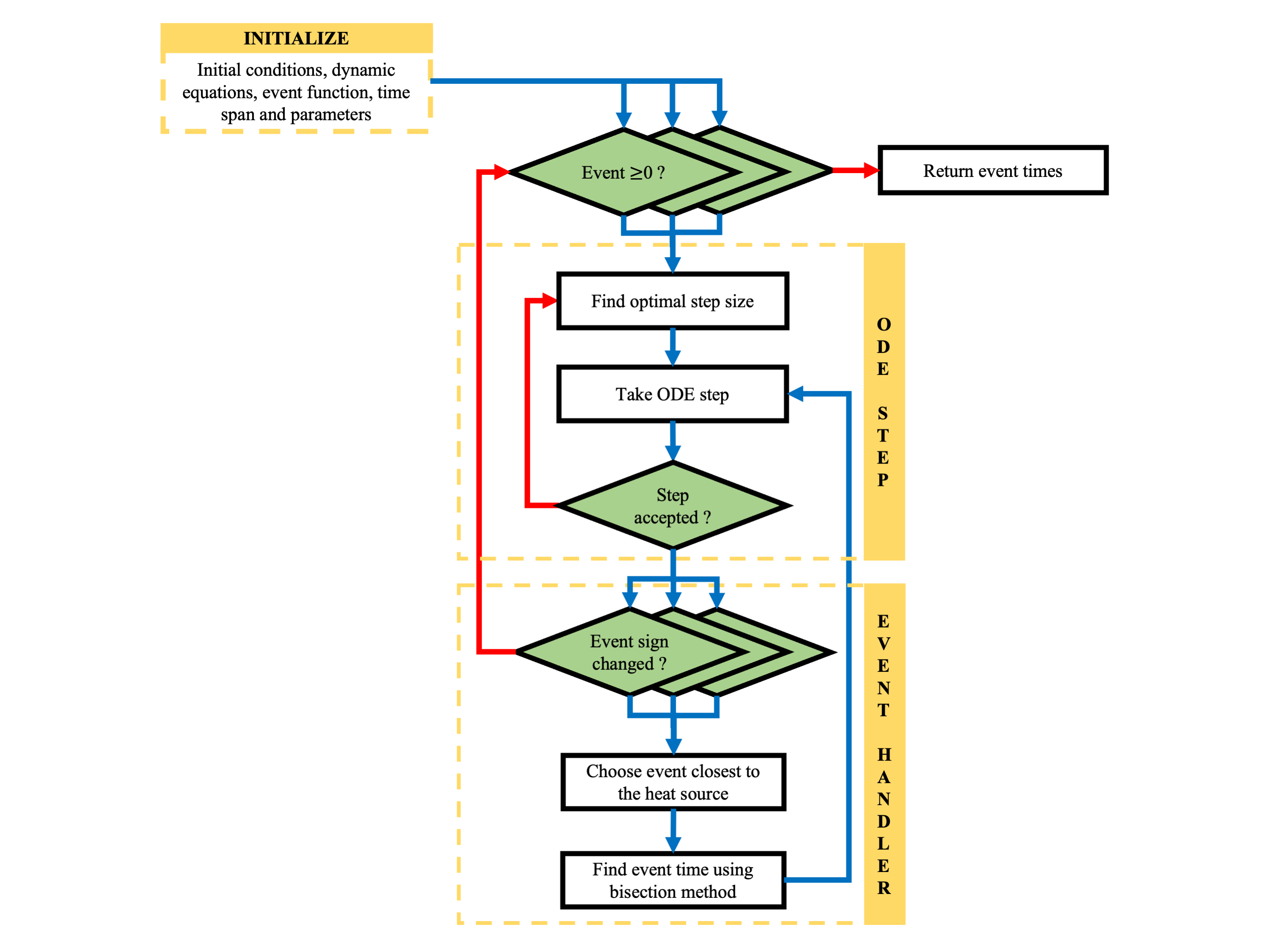
Notice that we have a custom_odeint_event function to determine the event times, which separates the two differential equations. We also ensure that its gradients are set to zero. In this function, to track events, we maintain a list of event times corresponding to each discretized point. The ODE solver proceeds by taking an ODE step and checking all events simultaneously. If multiple events are triggered at the next step, only the one closest to the bottom is selected. The event time is determined, the list is updated, and the previous ODE step is repeated with the updated list. This process continues until the remaining list is populated. A schematic of its working is shown below
def interp_fit_dopri(y0, y1, k, dt):
    # Fit a polynomial to the results of a Runge-Kutta step.
    dps_c_mid = jnp.array([
        6025192743 / 30085553152 / 2, 0, 51252292925 / 65400821598 / 2,
        -2691868925 / 45128329728 / 2, 187940372067 / 1594534317056 / 2,
        -1776094331 / 19743644256 / 2, 11237099 / 235043384 / 2])
    y_mid = y0 + dt*jnp.dot(dps_c_mid, k)
    return jnp.array(fit_4th_order_polynomial(y0, y1, y_mid, k[0], k[-1], dt))

def fit_4th_order_polynomial(y0, y1, y_mid, dy0, dy1, dt):
    a = -2.*dt*dy0 + 2.*dt*dy1 -  8.*y0 -  8.*y1 + 16.*y_mid
    b =  5.*dt*dy0 - 3.*dt*dy1 + 18.*y0 + 14.*y1 - 32.*y_mid
    c = -4.*dt*dy0 +    dt*dy1 - 11.*y0 -  5.*y1 + 16.*y_mid
    d = dt * dy0
    e = y0
    return a, b, c, d, e

def runge_kutta_step(afunc, y0, f0, t0, dt, *args):
    # Dpri5 Butcher Table
    c = jnp.array([1 / 5, 3 / 10, 4 / 5, 8 / 9, 1., 1., 0])
    a = jnp.array([
        [1 / 5, 0, 0, 0, 0, 0, 0],
        [3 / 40, 9 / 40, 0, 0, 0, 0, 0],
        [44 / 45, -56 / 15, 32 / 9, 0, 0, 0, 0],
        [19372 / 6561, -25360 / 2187, 64448 / 6561, -212 / 729, 0, 0, 0],
        [9017 / 3168, -355 / 33, 46732 / 5247, 49 / 176, -5103 / 18656, 0, 0],
        [35 / 384, 0, 500 / 1113, 125 / 192, -2187 / 6784, 11 / 84, 0]
    ])
    b = jnp.array([35 / 384, 0, 500 / 1113, 125 / 192, -2187 / 6784, 11 / 84, 0])
    b_error = jnp.array([
        35 / 384 - 1951 / 21600, 0, 500 / 1113 - 22642 / 50085,
        125 / 192 - 451 / 720, -2187 / 6784 - -12231 / 42400,
        11 / 84 - 649 / 6300, -1. / 60.
        ])

    def body_func(k, i):
        t1 = t0 + dt*c[i - 1]
        y1 = y0 + dt*jnp.dot(a[i - 1], k)
        f1 = afunc(y1, t1, *args)
        return k.at[i].set(f1), i

    k = jnp.zeros(shape = (7, len(y0))).at[0].set(f0)
    k, _ = jax.lax.scan(body_func, k, jnp.arange(1, 7))
    y1 = y0 + dt*jnp.dot(b, k)
    f1 = k[-1]
    y1_err = dt*jnp.dot(b_error, k)

    return y1, y1_err, k, f1

def initial_step_size(afunc, t0, y0, order, rtol, atol, f0, *args):
    # Algorithm from:
    # E. Hairer, S. P. Norsett G. Wanner,
    # Solving Ordinary Differential Equations I: Nonstiff Problems, Sec. II.4.
    scale = atol + jnp.abs(y0) * rtol
    d0 = jnp.linalg.norm(y0 / scale)
    d1 = jnp.linalg.norm(f0 / scale)

    h0 = jnp.where((d0 < 1e-5) | (d1 < 1e-5), 1e-6, 0.01 * d0 / d1)

    y1 = y0 + h0 * f0
    f1 = afunc(y1, t0 + h0, *args)
    d2 = jnp.linalg.norm((f1 - f0) / scale) / h0

    h1 = jnp.where((d1 <= 1e-15) & (d2 <= 1e-15),
                jnp.maximum(1e-6, h0 * 1e-3),
                (0.01 / jnp.max(d1 + d2)) ** (1. / (order + 1.)))

    return jnp.minimum(100. * h0, h1)

def mean_error_ratio(error_estimate, rtol, atol, y0, y1):
    err_tol = atol + rtol * jnp.maximum(jnp.abs(y0), jnp.abs(y1))
    err_ratio = error_estimate / err_tol.astype(error_estimate.dtype)
    return jnp.sqrt(jnp.mean(err_ratio**2))

def optimal_step_size(last_step, mean_error_ratio, safety=0.9, ifactor=10.0,
                      dfactor=0.2, order=5.0):
    """Compute optimal Runge-Kutta stepsize."""
    dfactor = jnp.where(mean_error_ratio < 1, 1.0, dfactor)

    """
    factor = jnp.minimum(ifactor,
                        jnp.maximum(mean_error_ratio**(-1.0 / order) * safety, dfactor))
    """

    factor = jnp.nanmin(jnp.array([ifactor,
                                 jnp.nanmax(jnp.array([mean_error_ratio**(-1.0 / order) * safety, dfactor]))]))

    return jnp.where(mean_error_ratio == 0, last_step * ifactor, last_step * factor)

@partial(jax.jit, static_argnums = (0, 1, 5, 6, 7))
def _custom_odeint_event(afunc, event, xinit, time_span, parameters, rtol, atol, mxstep = None):
    # Once all events are reached the forward simulation stops and the event time is output

    # This code is similar to
    # https://github.com/jacobjinkelly/easy-neural-ode/blob/master/lib/ode.py

    _afunc = lambda x, t, event_times : afunc(x, t, (event_times, parameters))
    _event_cond = lambda x, t : event(x, t) >= 0 # x - xcrit

    def scan_func(carry, target_t):

        def cond_func(state):
            # conditions to continue
            _, _, _, t, dt, *_, _events = state
            return (t < target_t) & (dt > 0) & (_events.any())

        def step_func(state):
            # body function if event has not reached yet
            i, y, f, t, dt, last_t, interp_coeff, event_times, events = state
            next_y, next_y_error, k, next_f = runge_kutta_step(_afunc, y, f, t, dt, event_times)
            next_t = t + dt
            error_ratios = mean_error_ratio(next_y_error, rtol, atol, y, next_y)
            new_interp_coeff = interp_fit_dopri(y, next_y, k, dt)
            dt = jnp.clip(optimal_step_size(dt, error_ratios), a_min = 0., a_max = jnp.inf)
            next_events = _event_cond(next_y, next_t)

            new = [i + 1, next_y, next_f, next_t, dt,      t, new_interp_coeff, event_times, next_events]
            old = [i + 1,      y,      f,      t, dt, last_t,     interp_coeff, event_times, events]
            return jax.lax.cond(jnp.all(error_ratios <= 1.), lambda : new, lambda : old)

        def find_event(state, new_state, counter, tol = 1e-8):
            # find event using bisection method

            i, prev_y, prev_f, prev_t, prev_dt, last_t, _interp_coeff, event_times, events = state
            _, next_y, _, next_t, _, _, next_interp_coeff, *_ = new_state

            _interp = lambda t : jnp.polyval(next_interp_coeff, (t - prev_t)/(next_t - prev_t))
            max_iter = jnp.ceil(jnp.log((next_t - prev_t)/tol)/jnp.log(2.))

            def body_func(carry):
                _cur_iter, _cur_y, _cur_t, _next_y, _next_t = carry
                mid_t = (_cur_t + _next_t)/2
                mid_y = _interp(mid_t)
                mid_events = _event_cond(mid_y, mid_t)

                left = [_cur_iter + 1, _cur_y, _cur_t, mid_y, mid_t]
                right = [_cur_iter + 1, mid_y, mid_t, _next_y, _next_t]

                return jax.lax.cond(mid_events[counter], lambda : right, lambda : left)

            def cond_func(carry):
                cur_iter, *_ = carry
                return cur_iter <= max_iter

            *_, _cur_t, _, _next_t = jax.lax.while_loop(cond_func, body_func, [0, prev_y, prev_t, next_y, next_t])

            # Make sure that the event times are unique
            _event_time = (_next_t + _cur_t) / 2
            event_times = event_times.at[counter].set(_event_time)
            # return previous state
            return [i, prev_y, prev_f, prev_t, prev_dt, last_t, _interp_coeff, event_times, events]

        def body_func(state):

            *_, event_times, _next_events = new_state = step_func(state)
            counters = jnp.argwhere(jnp.logical_not(_next_events) & (event_times == time_span[-1] + 1), size = xdim, fill_value = xdim).flatten()

            next_state = jax.lax.cond(
                counters[0] == xdim,
                lambda *args : args[1],
                find_event,
                state, new_state, counters[0]
            )
            return next_state

        # TODO get counter closest to heat source and whose event time is -1
        n_steps, *carry = jax.lax.while_loop(cond_func, body_func, [0] + carry)
        return carry, None

    xdim = xinit.shape[0]
    init_events = _event_cond(xinit, time_span[0])
    event_times = jnp.where(init_events, time_span[-1] + 1, time_span[0] - 1)
    f0 = _afunc(xinit, time_span[0], event_times)
    dt = initial_step_size(_afunc, time_span[0], xinit, 4, rtol, atol, f0, event_times)
    interp_coeff = jnp.array([xinit] * 5)
    init_carry = [xinit, f0, time_span[0], dt, time_span[0], interp_coeff, event_times, init_events]

    _time_span = jnp.array([time_span[0], time_span[-1]])
    carry, _ = jax.lax.scan(scan_func, init_carry, _time_span[1:])

    return carry[-2] # return event_times

@partial(jax.custom_jvp, nondiff_argnums = (0, 1, 5, 6, 7))
def custom_odeint_event(afunc, event, xinit, time_span, parameters, rtol, atol, mxstep = None):
    return jax.lax.stop_gradient(_custom_odeint_event(afunc, event, xinit, time_span, parameters, rtol, atol, mxstep))

@custom_odeint_event.defjvp
def custom_odeint_event_fwd(afunc, event, rtol, atol, mxstep, primals, tangents):
    xinit, time_span, parameters = primals
    event_times = custom_odeint_event(afunc, event, xinit, time_span, parameters, rtol, atol, mxstep)
    return event_times, jnp.zeros_like(event_times)
5. Example
Consider a 2D system that follows the dynamics bar before the event and the dynamics foo after the event is triggered. The condition that triggers the event is given by the event function.
# Function for single discretized point of x
def bar(x, t, p): return jnp.array([- p[0] * x[0], - p[0] * x[1]]) # Before event is triggered
def foo(x, t, p): return jnp.array([- p[0] * x[0]**2, - p[0] * x[1]**2]) # After event is triggered
def event(x, t): return jnp.array([x[0] - 1.]) # Event condition
# Functions vmapped over discretized points of x
def afunc(x, t, args):
event_times, p = args
return jax.vmap(lambda _x, _event : jax.lax.cond(t <= _event, lambda : bar(_x, t, p), lambda : foo(_x, t, p)))(x, event_times)
def transfer(trans_func, x, t, args): return trans_func(afunc, event, x, t, args) # Transfer function for sensitivity transfer
def event_vmap(x, t): return jax.vmap(event, in_axes = (0, None))(x, t)
# sorted event times
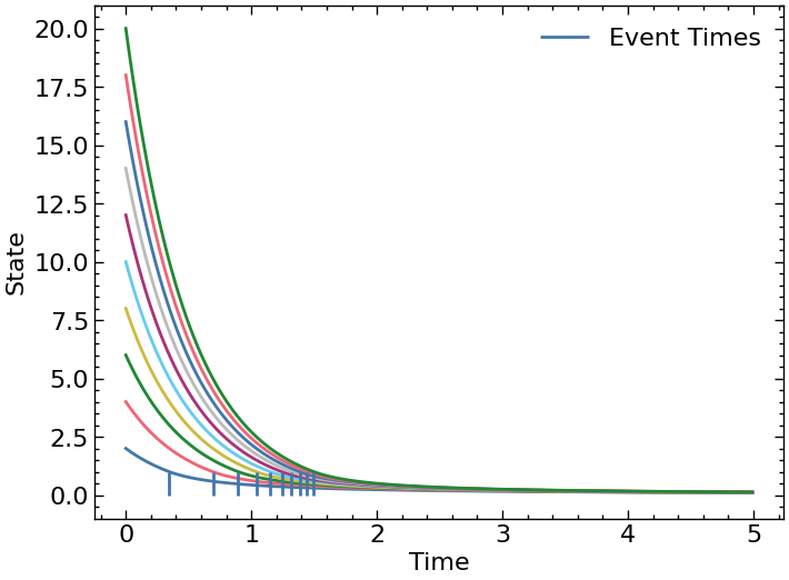
time_span = jnp.arange(0, 5., 0.01)
p = jnp.array([2.])
xinit = jnp.arange(2, 10. * 2 + 2).reshape(-1, 2) # shape = (Discretized points X dimension of x)
trajectory, event_times = odeint_event(afunc, event_vmap, transfer, xinit, time_span, p)
# permuted initial conditions
key = jrandom.PRNGKey(10)
permutation = jrandom.permutation(key, jnp.arange(xinit.shape[0]))
trajectory_permute, event_times_permute = odeint_event(afunc, event_vmap, transfer, xinit[permutation], time_span, p)
assert jnp.allclose(event_times[permutation], event_times_permute)
We will now create a dummy objective function and check our gradients using finite difference.
# checking automatic differentiation gradients with finite difference

def objective(x, t, p):
    time_span = jnp.linspace(0, t, 100)
    xinit = jnp.tile(x, (10, 1)) + jrandom.normal(key, shape = (10, 2)) * 0.1
    solution = odeint_event(afunc, event_vmap, transfer, xinit, time_span, p)
    return jnp.mean((solution[0])**2)


# check gradients using finite difference
def gradient_fd(x, t, p, eps):

    args_flatten, unravel = flatten_util.ravel_pytree(( x, t, p ))
    def _grad(v):
        loss = objective(*unravel(args_flatten + eps * v)) - objective(*unravel(args_flatten - eps * v))
        return loss / 2 / eps

    _gradients = jax.vmap(_grad)(jnp.eye(len(args_flatten)))
    return unravel(_gradients)


x = xinit[0]
t = jnp.array(5.)

# Testing gradients
gradient_x, gradient_t, gradient_p = jax.grad(objective, argnums = (0, 1, 2))(x, t, p) # reverse-mode autodiff compatible
gradient_x, gradient_t, gradient_p = jax.jacfwd(objective, argnums = (0, 1, 2))(x, t, p) # forward-mode autodiff compatible

eps = 1e-4
fd_x, fd_t, fd_p = gradient_fd(x, t, p, eps)

assert jnp.allclose(fd_x, gradient_x, atol = 100 * eps), "Finite difference does not match for x"
assert jnp.allclose(fd_p, gradient_p, atol = 100 * eps), "Finite difference does not match for p"
assert jnp.allclose(fd_t, gradient_t, atol = 100 * eps), "Finite difference does not match for t"
We can also compute the Hessian matrix, because the custom jvp rule is linear in tangent space.
# Testing hessians - forward-over-reverse mode autodiff
hess = jax.hessian(objective, argnums = (0, 1, 2))(x, t, p)
6. References
-
Siddharth Prabhu, Sulman Haque, Dan Gurr, Loren Coley, Jim Beilstein, Srinivas Rangarajan, and Mayuresh Kothare. An event-based neural partial differential equation model of heat and mass transport in an industrial drying oven. Computers Chemical Engineering, 200:109171, 2025. ↩
-
H. Zhang, S. Abhyankar, E. Constantinescu and M. Anitescu, “Discrete Adjoint Sensitivity Analysis of Hybrid Dynamical Systems With Switching,” in IEEE Transactions on Circuits and Systems I: Regular Papers, vol. 64, no. 5, pp. 1247-1259, May 2017, doi: 10.1109/TCSI.2017.2651683. ↩
-
Kidger, P., 2022. On neural differential equations arXiv:2202.02435. ↩
-
Diehl, M., Gros, S., 2011. Numerical optimal control. Optimization in Engineering Center (OPTEC) ↩