Siddharth Prabhu

Parameter Estimation, Optimal Control, Machine Learning, Optimization, Automatic Differentiation, System Identification

Hybrid Modeling of System Governed by Differential Equations

Introduction
Implementation in JAX
References

1. Introduction

Hybrid modeling is an emerging class of data-driven approach for modeling systems governed by differential equations. In this approach, a “simple” mechanistic model that sufficiently approximates the system’s dynamics is chosen. To make this “simple” mechanistic model felexible, a neural network is used either to estimate the parameters of this model or to provide corrective terms that account for unmodeled dynamics, using the system states as inputs. The neural network is then trained using experimental measurements of the states. Unlike the training approach used in physics-informed neural netoworks (PINN’s) ¹, which uses a neural network to approximate the states at different time points while the mechanistic model acts as soft constraint, this approach is trained with a mechanistic model in the loop. This ensures that the resulting model strictly adheres to physical laws and can generalize more effectively to unseen data. However, training can be computationally expensive. During the forward pass, a partial (or ordinary) differential equation is simulated, and during the backward pass, gradients are computed through this simulation. Consequently, each training iteration incurs a high computational cost. In this tutorial, we will explore a simple example of hybrid modeling for a dynamical system using JAX.

2. Implementation is JAX

We start by importing necessary Python packages. Basically we need a differentiable ODE solver and an optimizer to train our neural network.

import jax
jax.config.update("jax_enable_x64", True)
import jax.numpy as jnp
import jax.random as jrandom
from jax.example_libraries import optimizers
from jax.experimental.ode import odeint
import matplotlib.pyplot as plt

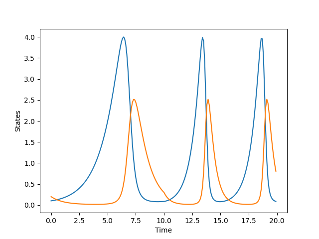
To generate data we will use the classic Lotka-Volterra system, the dynamics of which are given below

\[\begin{equation} \begin{aligned} \frac{dx}{dt} & = p_1 x - p_2 x y \\ \frac{dy}{dt} & = - p_3 y + p_4 x y \end{aligned} \end{equation}\]

with initial conditions $ x(t = 0) = 0.1, \ y(t = 0) = 0.2$, and time horizon as [$t_0 = 0, \ t_f = 20, \ \Delta t = 0.1$]. We will consider the parameters to be time dependant, given as follows

\[\begin{equation} \{ p_1, \ p_2, \ p_3, \ p_4 \} = \begin{cases} \{ 2/3, \ 4/3, \ 1, \ 1 \} & \text{if $t \leq 10$} \\ \{ 4/3, \ 8/3, \ 2, \ 2 \} & \text{otherwise} \end{cases} \end{equation}\]

We can then simulate these equations using JAX compatible ODE solver to get the target values as follows

def LotkaVolterra(x, t, p) : 
    """
    Lotka-Volterra dynamics with known parameters and their time dependance
    """
    p = jnp.where(t <= 10., p, 2 * p) # Time dependant parameters
    return jnp.array([
        p[0] * x[0] - p[1] * x[0] * x[1], 
        - p[2] * x[1] + p[3] * x[0] * x[1]
    ])

t = jnp.arange(0, 20., 0.1) # Time span
x = jnp.array([0.1, 0.2]) # Initial conditions
p = jnp.array([2/3, 4/3, 1, 1]) # parameters
target = odeint(LotkaVolterra, x, t, p) # Integrate

If we plot the target values, we observe the following trajectories

We will now define a function init_params that initializes the parameters of the neural network based on the dimensions of the input, output, and hidden layers. Additionally, we will define another function mlp that performs the forward pass given the inputs and network parameters, returning the network’s output. We use the ReLU activation function between hidden layers. Note that, since we want all parameters to be positive, we will apply an exponential function to the output layer.

def init_params(key : jnp.ndarray, dimensions : List, scale : float = 0.01) -> Dict[str, List[jnp.ndarray]]:
    """
    Initialize parameters that are normally distributed and scaled 
    """
    parameters = defaultdict(list)
    keys = jrandom.split(key, len(dimensions) - 1)
    for m, n, key in zip(dimensions[:-1], dimensions[1:], keys):
        key_weight, key_bias = jrandom.split(key, 2)
        sigma =  1./jnp.sqrt(m)
        parameters["weights"].append(scale * jrandom.uniform(key_weight, minval = -sigma, maxval = sigma, shape = (n, m)))
        parameters["bias"].append(scale * jrandom.uniform(key_bias, minval = -sigma, maxval = sigma, shape = (n, )))
    return parameters


def mlp(x, p):
    """
    Forward pass of neural network
    """
    n = len(p["weights"])
    for i, (weight, bias) in enumerate(zip(p["weights"], p["bias"])):
        x = jnp.dot(weight, x) + bias
        if i < n - 1 : # no activation on the last layer
            x = jnp.where(x <= 0, 0., x) # ReLU activation function
    return jnp.exp(x) # Making sure that the parameters are positive

Once we have defined these functions, we will proceed to define NeuralLotkaVolterra, which we will integrate to obtain the simulated trajectory. To ensure that the simulated trajectory closely matches the target values, we define an objective function that minimizes the squared loss. Note that the key difference between LotkaVolterra and NeuralLotkaVolterra is that, in the former, the parameters and their time dependence are known, whereas in the latter, the parameters are unknown and are instead predicted by a neural network that takes the time point $t$ as input.

def NeuralLotkaVolterra(x, t, pnn) : 
    """
    Lotka-Volterra dynamics with parameters given by a neural network
    """
    _p = mlp(jnp.atleast_1d(t), pnn)
    return jnp.array([
        _p[0] * x[0] - _p[1] * x[0] * x[1], 
        - _p[2] * x[1] + _p[3] * x[0] * x[1]
    ])

def objective(pnn, target):
    """
    Objective function
    """
    solution = odeint(NeuralLotkaVolterra, x, t, pnn)
    return jnp.mean((solution - target)**2)

We can observe a key difference between this approach and PINNs. In this approach, we still need to integrate the governing equations using an ODE solver, although with unknown parameters, thereby preserving the underlying physics. In contrast, PINNs do not require an ODE solver.

We have now completed the problem setup and can proceed to initialize and train our neural network. The input dimension of the network is $1$, as we only consider time as the input, while the output dimension is $4$, corresponding to the four parameters. The network has two hidden layers with dimensions $16$ and $32$, respectively. We will use the Adam optimizer with a learning rate of $0.001$, which will be reduced to $0.0001$ after $5000$ iterations. To compute gradients, we will use the jax.value_and_grad function.

key = jrandom.PRNGKey(20)
pinit = init_params(key, dimensions = [1, 16, 32, 4])
lr = 0.001
max_iter = 10000
opt_init, opt_update, get_params = optimizers.adam(optimizers.piecewise_constant([5000], [lr, 0.1 * lr]))
opt_state = opt_init(pinit)
get_grads = jax.jit(jax.value_and_grad(objective))

We then train for $10^{4}$ iterations

for iteration in range(max_iter):
    pnn = get_params(opt_state)
    loss, pnn_grad = get_grads(pnn, solution)
    opt_state = opt_update(iteration, pnn_grad, opt_state)
    print(f"Iteration : {iteration}, Objective : {loss}")

At the end of training we get a loss of $9 \times 10^{-3}$. We compare the traget trajectories and predicted trajectories below.

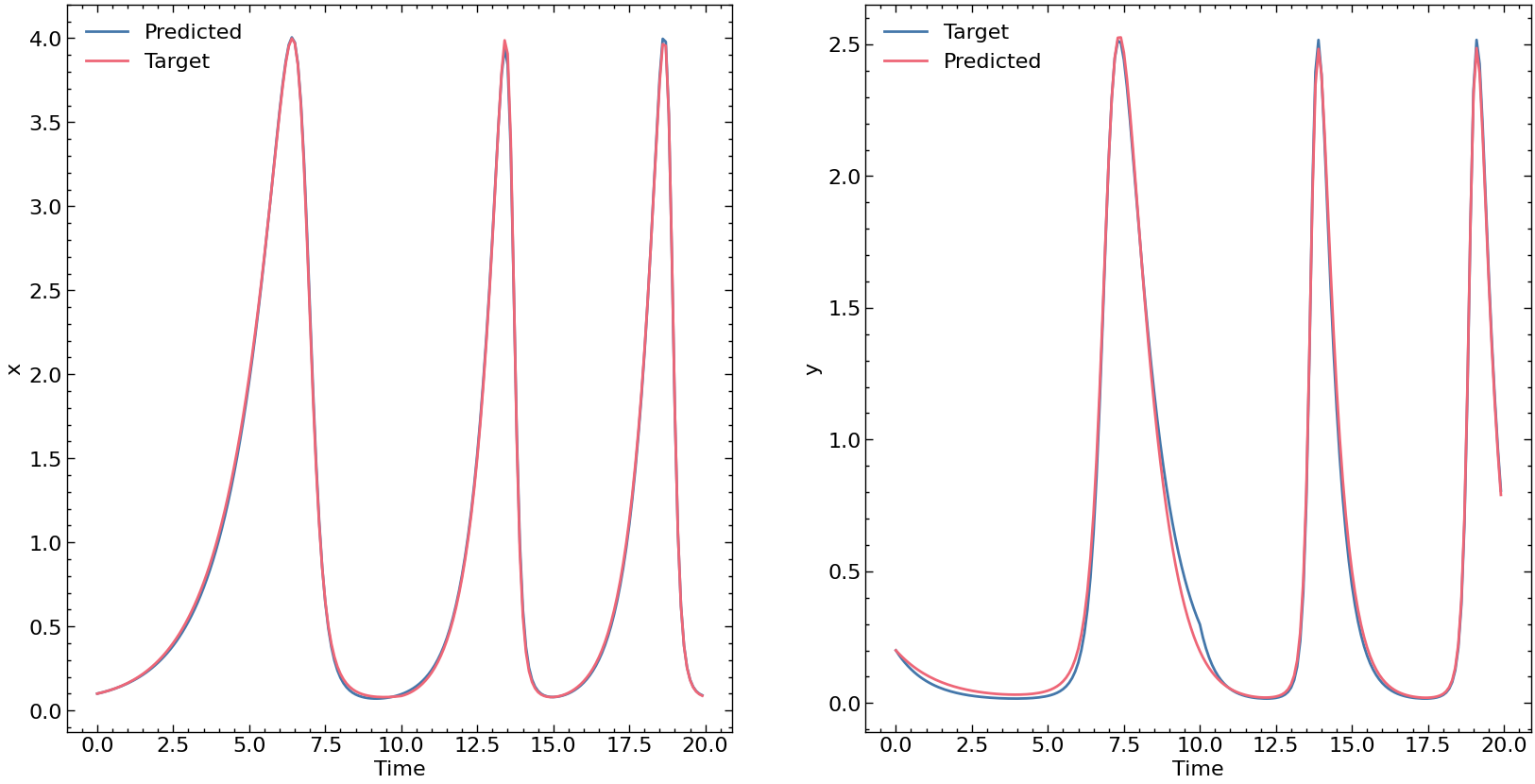
Note that this is still a simplified example using synthetic data. A more complex case, involving a hybrid partial differential equation and real industrial data, is presented in our paper ².

Siddharth Prabhu

Hybrid Modeling of System Governed by Differential Equations

Table of Contents

1. Introduction

2. Implementation is JAX

3. References