Siddharth Prabhu

Parameter Estimation, Optimal Control, Machine Learning, Optimization, Automatic Differentiation, System Identification

Differentiable Dynamic Programming with Constraints Using Interior-Point Method

Introduction
Unconstrained Differential Dynamic Programming
Constrained Differential Dynamic Programming
1. Regularization
2. Algorithm
Car Obstacle Avoidance Example
References

1. Introduction

One of the popular algorithms to solve an optimal control problem in recent times, is called Differential Dynamic Programming (DDP) ¹. It is an dynamic programming based approach that finds the optimal control law by minimizing the quadratic approximation of the value function. DDP in its original form does not admit state and control constraints. There have been several extensions to overcome this drawback, and most of them, if not all, fall into three major classes of solution techniques - augmented lagrangian methods, active set methods, and barrier methods. All of these methods essentially solve a two-layer optimization problem. In this tutorial, we will look at the interior point differential dynamic programming proposed in ² for handling stagewise equality and inequality constraints.

2. Unconstrained Differential Dynamic Programming

Consider a discrete-time dynamical system

\[\begin{equation} x_{k + 1} = f(x_k, u_k) \end{equation}\]

where $x_k \in \mathbb{R}^n$ and $u_k \in \mathbb{R}^m$ are the states and control inputs at time $k$. The function $f : \mathbb{R}^n \times \mathbb{R}^m \rightarrow \mathbb{R}^n$ describes the evolution of the states to time $k + 1$ given the states and control inputs at time $k$. Consider a finite time optimal control problem starting at initial state $x_0$

\[\begin{equation} \begin{aligned} J^*(\textit{X}, \textit{U}) & = \min _{\textit{U}} \sum _{k = 0}^{N - 1} l(x_k, u_k) + l_f(x_N) \\ \text{subject to} & \\ & \quad x_{k + 1} = f(x_k, u_k) \end{aligned} \end{equation}\]

where the scalar-valued functions $l, l_f, J$ denote the running cost, terminal cost, and total cost respectively. $\textit{X} = (x_0, x_1, …, x_N)$ and $ \textit{U} = (u_0, u_1, …, u_{N - 1})$ are the sequence of state and control inputs over the control horizon $N$. We can solve this problem using dynamic programming. If we define the optimal value function at time $k$ as

\[\begin{equation} V_k(x_k) = \min _{u_k} \left[ l(x_k, u_k) + V_{k + 1}(x_{k + 1}) \right] \end{equation}\]

then, starting from $V_N(x_N) = l_f(x_N)$, the solution to the finite time optimal control problem in equation 2 boils down to finding $V_0$. At every time step $k$, differential dynamic programming solves the optimization problem in equation 3 using a quadratic approximation of the value function. The value function is approximated around the states obtained by integrating equation 1 for given control inputs. Let $Q(x_k + \delta x_k, u_K + \delta u_k)$ be the second order Taylor series approximation of (\ref{eqn:val-fun}) around the point $x_k$ and $u_k$. Then the above equation after dropping the subscript $k$ for simplicity, can be written as

\[\begin{equation} V_k(x) = \min _{\delta u} Q + \begin{bmatrix} Q_x \\ Q_u \end{bmatrix}^T \begin{bmatrix} \delta x \\ \delta u\end{bmatrix} + \frac{1}{2} \begin{bmatrix} \delta x \\ \delta u \end{bmatrix}^T \begin{bmatrix} Q_{xx} & Q_{xu} \\ Q_{ux} & Q_{uu} \end{bmatrix} \begin{bmatrix} \delta x \\ \delta u \end{bmatrix} \end{equation}\]

where

\[\begin{equation} \begin{aligned} & Q = l + V \\ & Q_x = l_x + f_x^TV_x \\ & Q_u = l_u + f_u^TV_x \\ & Q_{xx} = l_{xx} + f_x^TV_{xx}f_x + V_x f_{xx} \\ & Q_{xu} = l_{xu} + f_x^TV_{xx}f_u + V_x f_{xu} \\ & Q_{ux} = l_{ux} + f_u^TV_{xx}f_x + V_x f_{ux} \\ & Q_{uu} = l_{uu} + f_u^TV_{xx}f_u + V_x f_{uu} \\ \end{aligned} \end{equation}\]

By taking the derivatives with respect to $\delta u$ and equating to zero, we get a locally linear feedback policy

\[\begin{equation} \begin{aligned} & Q_{uu} \delta u + Q_u + Q_{ux} \delta x = 0 \\ & \delta u = - Q_{uu}^{-1} [Q_u + Q_{ux} \delta x] \end{aligned} \end{equation}\]

This is equivalent to solving the quadratic approximation of the following optimization problem at time point $k$

\[\begin{equation} \min _{x_k, u_k} l(x_k, u_k) + V_{k + 1}(f(x_k, u_k)) \end{equation}\]

which results in the following KKT conditions, after dropping the subscript $k$ for simplicity

\[\begin{equation} \begin{bmatrix} l_x + f_x^TV_x \\ l_u + f_u^TV_x \end{bmatrix} = 0 \end{equation}\]

Since the subproblem is quadratic, we can obtain the solution using one Newton step given by the following set of equations

\[\begin{equation} \begin{bmatrix} l_{xx} + f_x^TV_{xx}f_x + V_x f_{xx} & l_{xu} + f_x^TV_{xx}f_u + V_x f_{xu} \\ l_{ux} + f_u^TV_{xx}f_x + V_x f_{ux} & l_{uu} + f_u^TV_{xx}f_u + V_x f_{uu} \end{bmatrix} \begin{bmatrix} \delta x \\ \delta u \end{bmatrix} = - \begin{bmatrix} l_x + f_x^TV_x \\ l_u + f_u^TV_x \end{bmatrix} \end{equation}\]

However instead of taking a step in both $\delta x$ and $\delta u$ direction, a step is taken only in $\delta u$ direction

\[\begin{equation} \delta u = - \left [ l_{uu} + f_u^TV_{xx}f_u + V_x f_{uu} \right]^{-1} \left [ l_u + f_u^TV_x + ( l_{ux} + f_u^TV_{xx}f_x + V_x f_{ux} ) \delta x \right] \end{equation}\]

Using the definition in equation 5, we arrive at the same equation for $\delta u$ as in equation 6.

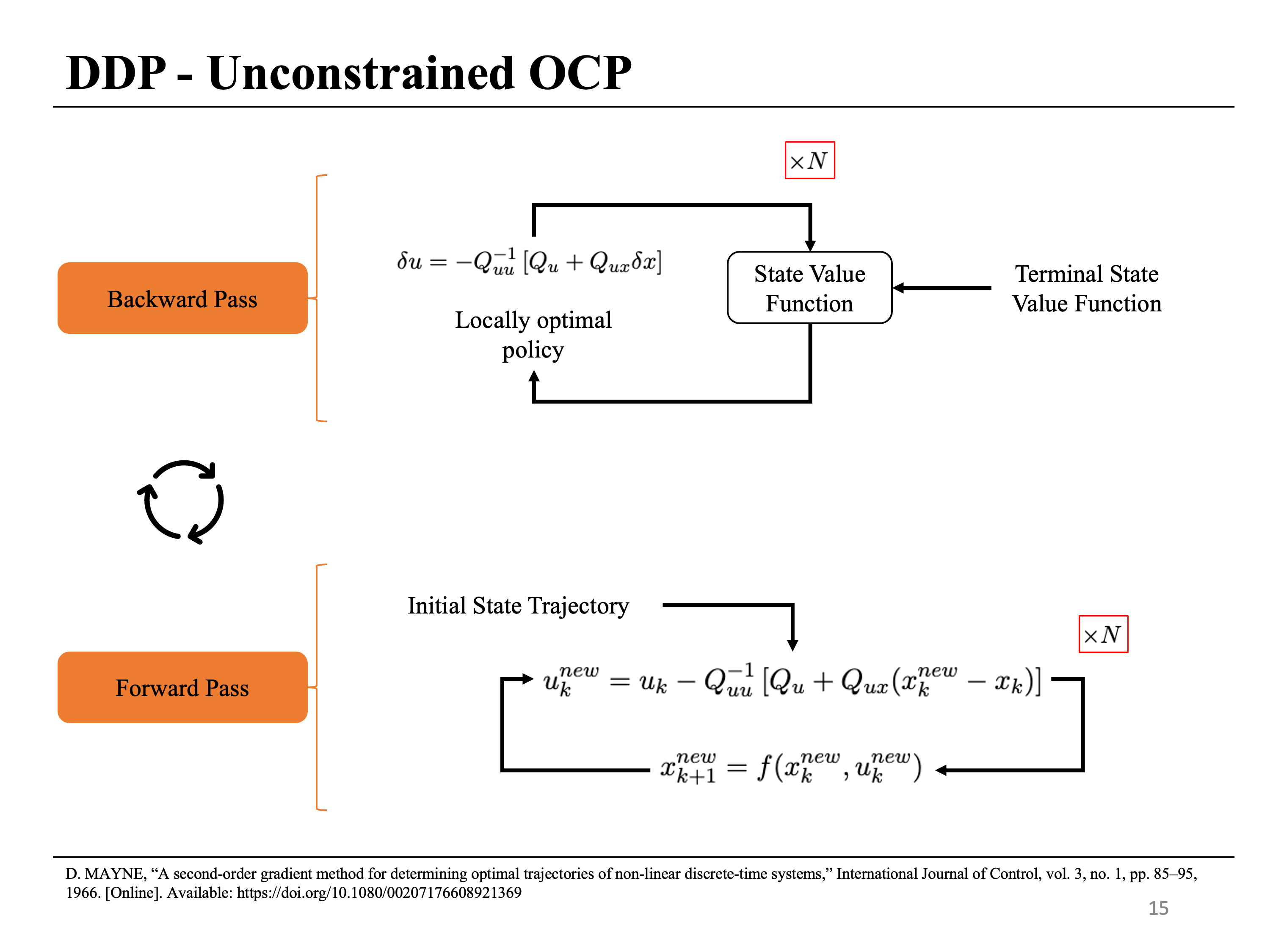
The equations 5 are propagated backward in time starting with the terminal cost and its derivatives. The backward pass gives an update rule for the control inputs as a function of states. The forward pass is then used to get the new state and control sequence for the next iteration. The procedure is repeated until some convergence criterion is reached.

\[\begin{equation} \begin{aligned} & V(x_N) = l_N \\ & V_x(x_N) = l_{N_x}(x_N) \\ & V_{xx}(x_N) = l_{N_{xx}}(x_N) \\ \end{aligned} \end{equation}\]

A pictorial representation of the forward and the backward pass is shown below

3. Constrainted Differential Dynamic Programming

Now, consider a constrained finite time optimal control problem starting at initial state $x_0$

\[\begin{equation} \begin{aligned} J^*(\textit{X}, \textit{U}) & = \min _{\textit{U}} \sum _{k = 0}^{N - 1} l(x_k, u_k) + l_f(x_N) \\ \text{subject to} & \\ & x_{k + 1} = f(x_k, u_k) \quad \forall \ k \in \{ 0, 1, \cdots N - 1 \} \\ & g_k (x_k, u_k) = 0 \quad \forall \ k \in \{ 0, 1, \cdots N - 1 \} \\ & h_k (x_k, u_k) \leq 0 \quad \forall \ k \in \{ 0, 1, \cdots N - 1 \} \\ & g_N (x_N) = 0 \\ & h_N (x_N) \leq 0 \\ \end{aligned} \end{equation}\]

with equality constraints $g_k (x_k, u_k)$ and inequality constraints $h_k (x_k, u_k)$ at every time step $k$. We add slack variables to convert the inequality constraints to equality constraints and require that the slack variables $s_k$ be positive. Another advantage of adding slack variables is that we can have an infeasible or arbitrary initial trajectory. An interior point algorithm is used to solve a sequence of barrier subproblems that eventually converge to the local optimum of the original unconstrained problem. The barrier subproblem that we solve is as follows

\[\begin{equation} \begin{aligned} J^*(\textit{X}, \textit{U}, \tau) & = \max _ {\Lambda} \min _{\textit{U}, \textit{M}} \sum _{k = 0}^{N - 1} \left[ l(x_k, u_k) + \lambda _k^T g_k(x_k, u_k) + \frac{\tau}{s_k} (h_k(x_k, u_k) + s_k) - \tau (1^T \log(s_k)) \right ] \\ & + \left[ l_f(x_N) + \lambda _N^T g_N(x_N) + \frac{\tau}{s_N} (h(x_N) + s_N) - \tau (1^T \log(s_N)) \right]\\ \text{subject to} & \\ & x_{k + 1} = f(x_k, u_k) \quad \forall \ i \in \{ 0, 1, \cdots N - 1 \} \\ & s_{k} \geq 0 \quad \forall \ i \in \{ 0, 1, \cdots N \} \end{aligned} \end{equation}\]

where $\tau$ is the barrier parameter, $\textit{M} = {s_0, s_1, …, s_N }$ are the slack variables and $\Lambda = { \lambda _0, \lambda _1, … \lambda _N }$ are the lagrange variables corresponding to the equality constraints $g(x_k, u_k)$. We can again apply dynamic programming to this problem by defining the value function as

\[\begin{equation} V_k(x_k) = \min _{u_k, s_k \geq 0} \max_{\lambda _k} \left[ l(x_k, u_k) + \lambda _k^T g_k(x_k, u_k) + \frac{\tau}{s_k} (h_k(x_k, u_k) + s_k) - \tau (1^T \log(s_k)) + V_{k + 1}(x_{k + 1}) \right] \end{equation}\]

To get the DDP update, we solve a similar optimization problem by defining $z_k = [x_k, u_k]$

\[\begin{equation} V_k(x_k) = \min _{z_k, s_k \geq 0} \max_{\lambda _k} \left[ l(x_k, u_k) + \lambda _k^T g_k(x_k, u_k) + \frac{\tau}{s_k} (h_k(x_k, u_k) + s_k) - \tau (1^T \log(s_k)) + V_{k + 1}(x_{k + 1}) \right] \end{equation}\]

which has the following KKT conditions, after dropping the subscript k for simplicity

\[\begin{equation} \begin{bmatrix} V_z \\ V_{\lambda} \\ V_s \end{bmatrix} = \begin{bmatrix} l_z + \lambda ^T g_z + \tau S^{-1} h_z + f_z^TV_z\\ g \\ h + s \end{bmatrix} = 0 \end{equation}\]

and requires the following Newton step

\[\begin{equation} \begin{aligned} \begin{bmatrix} l_{zz} + \lambda ^T g_{zz} + \tau S^{-1} h_{zz} + f_z^TV_{zz}f_z + V_z f & g_z ^T & h_z ^ T S^{-2} \tau\\ g_z & 0 & 0\\ h_z & 0 & I \end{bmatrix} \begin{bmatrix} \delta z \\ \delta \lambda \\ \delta s \end{bmatrix} = - \begin{bmatrix} l_z + \lambda ^T g_z + \tau S^{-1} h_z + f_z^TV_z\\ g \\ h + s \end{bmatrix} \end{aligned} \end{equation}\]

Regularization

Let $B_{zz} = l_{zz} + \lambda ^T g_{zz} + \frac{\tau}{s} h_{zz} + f_z^TV_{zz}f_z + V_z f$, $B_{z} = l_z + \lambda ^T g_z + \frac{\tau}{s} h_z + f_z^TV_z $, and $S = diag(s)$. Because we maximize with respect to the lagrange variables $\lambda $, we add a negative definite regularization as a function of the barrier parameter $T = \epsilon (\tau) *I$ to the Hessian matrix. The updated system of equations are

\[\begin{equation} \begin{bmatrix} B_{zz} & g_z ^T & - h_z ^ T S^{-2} \tau\\ g_z & - \mathrm{T} & 0\\ h_z & 0 & I \end{bmatrix} \begin{bmatrix} \delta z \\ \delta \lambda \\ \delta s \end{bmatrix} = - \begin{bmatrix} B_z\\ g \\ h + s \end{bmatrix} \end{equation}\]

Eliminating the last two rows gives the following equation for z

\[\begin{equation} \begin{bmatrix} B_{zz} + h_z ^ T \tau S^{-2} h_z + g_z^T \mathrm{T}^{-1} g_z\\ \end{bmatrix} \begin{bmatrix} \delta z \\ \end{bmatrix} = - \begin{bmatrix} B_z + h_z ^ T \tau S^{-2} h + h_z^T \tau S^{-1} + g_z^T \mathrm{T}^{-1} g\\ \end{bmatrix} \end{equation}\]

and the other variables are given as

\[\begin{equation} \begin{aligned} & \delta \lambda = \mathrm{T}^{-1} [ g + g_z \delta z ] \\ & \delta s = - I^{-1} [h + s + h_z \delta z] \end{aligned} \end{equation}\]

Substituting for $z$ gives

\[\begin{equation} \begin{bmatrix} B_{xx} + h_x ^ T \tau S^{-2} h_x + g_x^T \mathrm{T}^{-1} g_x & B_{xu} + h_x^T \tau S^{-2} h_u + g_x^T \mathrm{T}^{-1} g_u\\ B_{ux} + h_u ^ T \tau S^{-2} h_x + g_u^T \mathrm{T}^{-1} g_x & B_{uu} + h_u^T \tau S^{-2} h_u + g_u^T \mathrm{T}^{-1} g_u\\ \end{bmatrix} \begin{bmatrix} \delta x \\ \delta u \end{bmatrix} = - \begin{bmatrix} B_x + h_x ^ T \tau S^{-2} h + h_x^T \tau S^{-1} + g_x^T \mathrm{T}^{-1} g\\ B_u + h_u ^ T \tau S^{-2} h + h_u^T \tau S^{-1} + g_u^T \mathrm{T}^{-1} g\\ \end{bmatrix} \end{equation}\]

Comparing the above equation with equation 9 and equation 5, we get the following values for the quadratic subproblem

\[\begin{equation} \begin{aligned} & \hat{Q} = l + V + \lambda ^T g + \tau S^{-1} (h + s) - \tau 1^T \log(s) \\ & \hat{Q}_x = l_x + f_x^TV_x + \tau S^{-1}h_x + \lambda ^T g_x + h_x ^ T \tau S^{-2} h + h_x^T \tau S^{-1} + g_x^T \mathrm{T}^{-1} g\\ & \hat{Q}_u = l_u + f_u^TV_x + \tau S^{-1}h_x + \lambda ^T g_x + h_u ^ T \tau S^{-2} h + h_u^T \tau S^{-1} + g_u^T \mathrm{T}^{-1} g\\ & \hat{Q}_{xx} = l_{xx} + f_x^TV_{xx}f_x + V_x f_{xx} + \lambda ^T g_{xx} + \tau S h_{xx} + h_x ^ T \tau S^{-2} h_x + g_x^T \mathrm{T}^{-1} g_x \\ & \hat{Q}_{xu} = l_{xu} + f_x^TV_{xx}f_u + V_x f_{xu} + \lambda ^T g_{xu} + \tau S h_{xu} + h_x ^ T \tau S^{-2} h_u + g_x^T \mathrm{T}^{-1} g_u\\ & \hat{Q}_{ux} = l_{ux} + f_u^TV_{xx}f_x + V_x f_{ux} + \lambda ^T g_{ux} + \tau S h_{ux} + h_u ^ T \tau S^{-2} h_x + g_u^T \mathrm{T}^{-1} g_x\\ & \hat{Q}_{uu} = l_{uu} + f_u^TV_{xx}f_u + V_x f_{uu} + \lambda ^T g_{uu} + \tau S h_{uu} + h_u ^ T \tau S^{-2} h_u + g_u^T \mathrm{T}^{-1} g_u\\ \end{aligned} \end{equation}\]

To use the control policy equation in 6, $\hat{Q}_{uu}$ should be positive definite. In addition to the global regularization $\mu _1$ proposed in ³, we also add a local regularization $\mu _2$ at every state. All algorithms use the following equations

\[\begin{equation} \begin{aligned} & \tilde{Q}_{xx} = \hat{Q}_{xx} + \mu _2 I \\ & \tilde{Q}_{ux} = \hat{Q}_{ux} + f_u^T (\mu _1 I ) f_x \\ & \tilde{Q}_{xu} = \hat{Q}_{xu} + f_x^T (\mu _1 I ) f_u \\ & \tilde{Q}_{uu} = \hat{Q}_{uu} + f_u^T (\mu _1 I) f_u + \mu _2 I \\ & k = - \tilde{Q}^{-1}_{uu} \hat{Q}_u \\ & K = - \tilde{Q}^{-1}_{uu} \hat{Q}_{ux} \end{aligned} \end{equation}\]

with the same value function updates for intermediate time steps

\[\begin{equation} \begin{aligned} & V = \hat{Q} + \frac{1}{2} k^T \hat{Q}_{uu} k + k^T \hat{Q}_u \\ & V_{x} = \hat{Q}_{x} + K^T \hat{Q}_{uu} k + K^T \hat{Q}_u + \hat{Q}_{ux}^T k \\ & V_{xx} = \hat{Q}_{xx} + K^T \hat{Q}_{uu} K + K^T \hat{Q}_{ux} + \hat{Q}_{ux}^T K \\ \end{aligned} \end{equation}\]

and value function updates for terminal step

\[\begin{equation} \begin{aligned} V_N & = l_N + \lambda _N^T g_N + \tau S_N^{-1} (h_N + s_N) - \tau 1^T \log(s_N) \\ V_{N_x} & = l_{x_N} + h_{x_N} ^ T \tau S_N^{-2} h_N + h_{x_N}^T \tau S_N^{-1} + g_{x_N}^T \mathrm{T}^{-1} g_N \\ V_{N_{xx}} & = l_{xx_N} + \lambda _N^T g_{xx_N} + \tau S_N h_{xx_N} + h_{x_N} ^ T \tau S_N^{-2} h_{x_N} + g_{_N}^T \mathrm{T}^{-1} g_{x_N} \\ \end{aligned} \end{equation}\]

Algorithm

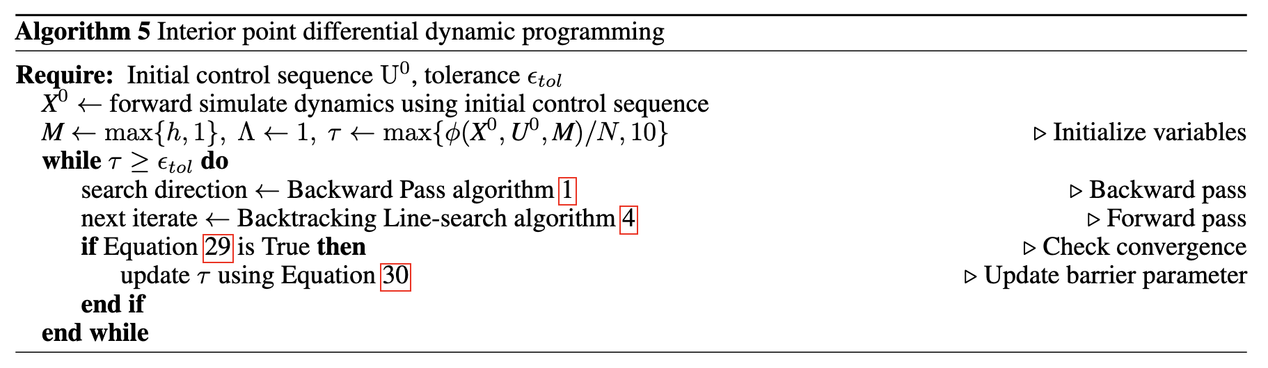
A pseudo code of the proposed algorithm is given below. We aim to solve a constrained optimal control problem. We address this by solving a series of barrier subproblems with a given value of the barrier parameter, which is decreased after the convergence criteria for each subproblem are met. Each barrier subproblem is solved using a DDP-like approach. The backward pass of DDP provides the update rule while the forward pass provides the next iterates. More information on backtracking line search and convergence criteria can be found in our paper.

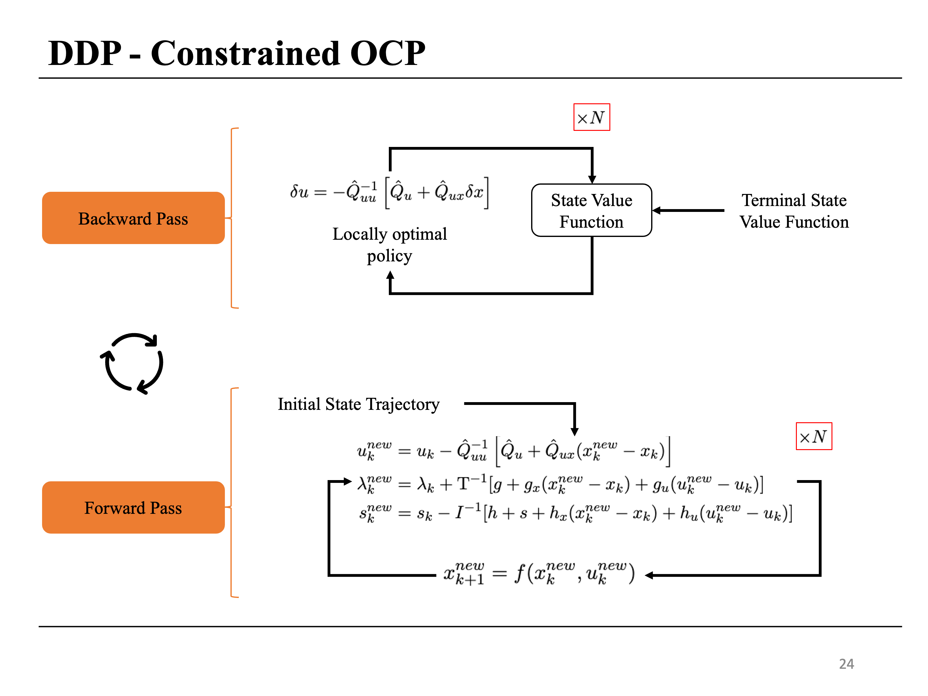
A pictorial representation of the forward and the backward pass is shown below

4. Car Obstacle Avoidance Example

We import the necessary packages

from typing import NamedTuple, Callable

import jax
jax.config.update("jax_enable_x64", True)
import jax.numpy as jnp
import jax.random as jrandom

from ilqr import iterative_linear_quadratic_regulator, TotalCost # Custom Functions

We will not go through the implementation of iterative_linear_quadratic_regulator function here. However, more details can be found on my GitHub

We consider a 2D car with the following dynamics

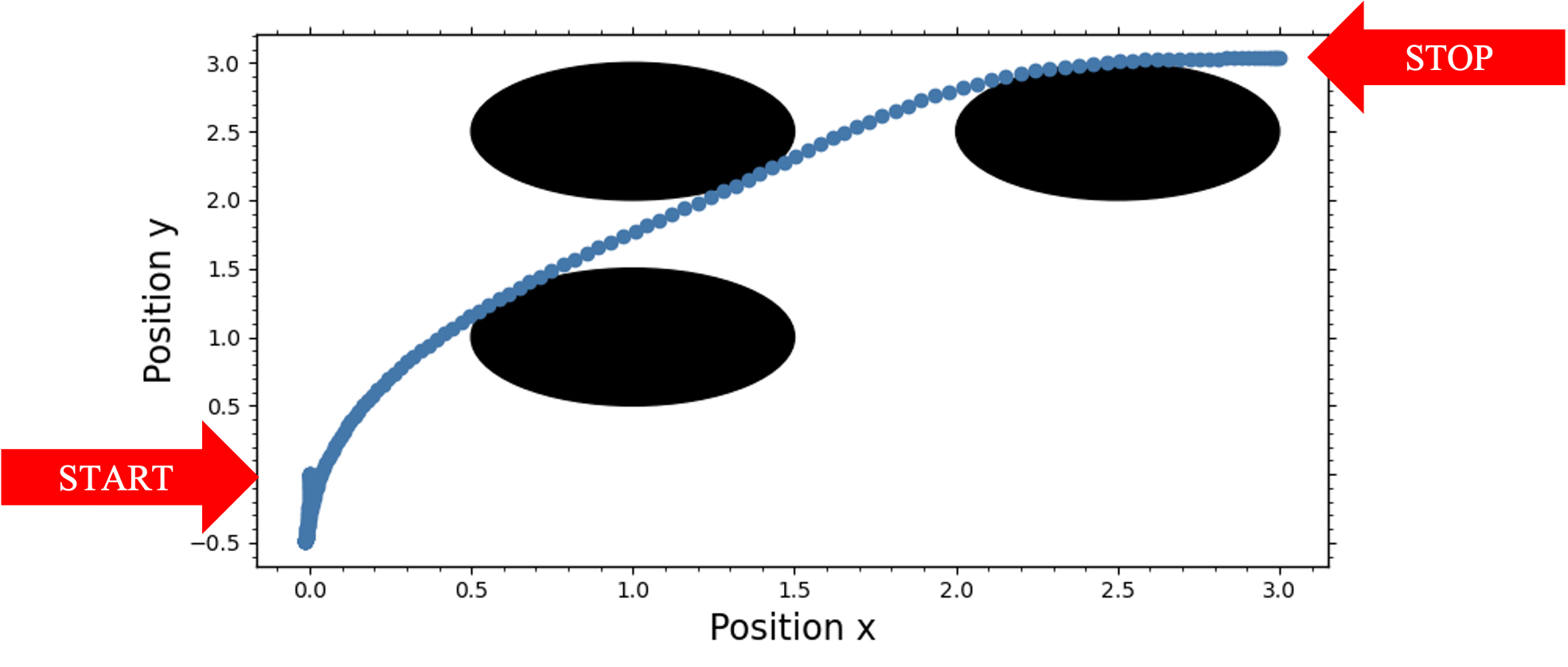
\[\begin{equation} f(x, u) = \begin{bmatrix} x_0 + h x_3 \sin{x_2} \\ x_1 + hx_3 \cos{x_2} \\ x_2 + h u_1 x_3 \\ x_3 + h u_0 \end{bmatrix} \end{equation}\]

where the states $x = [x_0, x_1, x_2, x_3]$ and the control inputs $u = [u_0, u_1]$. Given the initial conditions $x = [0, 0, 0, 0]$, the goal is to reach the terminal state $x(T) = [3, 3, \pi/2 0] $ using control inputs that are bounded using inequality constraints $ \pi / 2 \leq u_0 \leq \pi /2 $, $ -10 \leq u_1 \leq 10 $ and avoiding three obstacles defined using the following inequality constraints

\[\begin{equation} \begin{aligned} 0.5^2 - (x_0 - 1)^2 - (x_1 - 1)^2 \leq 0 \\ 0.5^2 - (x_0 - 1)^2 - (x_1 - 2.5)^2 \leq 0 \\ 0.5^2 - (x_0 - 2.5)^2 - (x_1 - 2.5)^2 \leq 0 \end{aligned} \end{equation}\]

The initial guess from control inputs is chosen uniformly between $[-0.01, 0.01]$ and a control horizon of $N = 200$ is chosen. We define the dynamics, running cost, terminal cost and the inequality constraints as follows

class CarObstacleExampleDynamics(NamedTuple):
    dt: float = 0.05
    
    def __call__(self, x, u, k = None):
        
        return jnp.array([
            x[0] + self.dt * x[3] * jnp.sin(x[2]), 
            x[1] + self.dt * x[3] * jnp.cos(x[2]),
            x[2] + self.dt * u[1] * x[3],
            x[3] + self.dt * u[0]
            ])


class CarObstacleExampleRunningCost(NamedTuple):
    q : jnp.ndarray = 0 * jnp.eye(4)
    r : jnp.ndarray = 0.05 * jnp.eye(2)

    def __call__(self, x, u, k = None):
        return x.T @ self.q @ x + u.T @ self.r @ u


class CarObstacleExampleTerminalCost(NamedTuple):
    q : jnp.ndarray = jnp.diag(jnp.array([50, 50, 50, 10.]))
    target : jnp.ndarray = jnp.array([3, 3, jnp.pi / 2, 0.])

    def __call__(self, x):
        _x = x - self.target
        return _x.T @ self.q @ _x


class CarObstacleExampleInequalityConstraints(NamedTuple):
    # inequality constraints of the form h(x, u) <= 0

    def __call__(self, x, u, k = None):
        return jnp.array([
            u[0] - jnp.pi / 2,
            - jnp.pi / 2 - u[0],
            u[1] - 10, 
            - 10 - u[1],
            0.5**2 - (x[0] - 1)**2 - (x[1] - 1)**2,
            0.5**2 - (x[0] - 1)**2 - (x[1] - 2.5)**2,
            0.5**2 - (x[0] - 2.5)**2 - (x[1] - 2.5)**2
        ])

We can now define and solve the optimal control problem

N = 200
dt = 0.05
x0 = jnp.array([0., 0., 0., 0.])
key = jrandom.PRNGKey(seed = 40)
u_guess = 0.001 * jrandom.randint(key, (N, 2), minval = -10, maxval = 10)

solution, total_time = iterative_linear_quadratic_regulator(
        CarObstacleExampleDynamics(dt), 
        TotalCost.form_cost(
            CarObstacleExampleRunningCost(), 
            terminal_cost = CarObstacleExampleTerminalCost(), 
            running_inequality_constraints_cost = CarObstacleExampleInequalityConstraints(),
            terminal_inequality_constraints_cost = None, 
            running_equality_constraints_cost = None,
            terminal_equality_constraints_cost = None
        ), 
        x0, u_guess, maxiter = 1000, atol = 1e-4, approx_hessian = False
    )

The algorithm successfully converges and produces a trajectory that avoids all the obstacles as shown below