BiLevel Optimization for Parameter Estimation of ODE in JAX
Table of Contents
1. Introduction
This tutorial introduces a bilevel optimization method for parameter estimation of ordinary differential equations based on our work in 1. A parameter estimation problem is an optimization problem
\[\begin{equation} \begin{aligned} & \min _{p} L(x(p), \ p) \quad \rightarrow \text{Objective function} \\ \text{subject to} & \\ & x(t = 0) = x_0 \quad \rightarrow \text{Given initial condition}\\ & \frac{dx}{dt} = f(x, p) \quad \rightarrow \text{Dynamic equation}\\ & g(p) = 0 \quad \rightarrow \text{Equality constraints}\\ & h(p) \leq 0 \quad \rightarrow \text{Inequality constraints} \end{aligned} \end{equation}\]where $x \in \mathbb{R}^n$ are the states, $p \in \mathbb{R}^p$ are the unknown parameters, $f(x, p) : \mathbb{R}^n \times \mathbb{R}^p \mapsto \mathbb{R}^n$ is the dynamic equation, $g(p) : \mathbb{R}^p \mapsto \mathbb{R}^g$ and $h(p) : \mathbb{R}^p \mapsto \mathbb{R}^h$ are the equality and the inequality constraints on the parameters. The objective function $L : \mathbb{R}^n \times \mathbb{R}^p \mapsto \mathbb{R}$ minimizes the experimental and the simulated trajectories. Ultimately the goal is to find the parameters that best describe the experimental measurements.
2. Method
This approach builds upon the method developed in DF-SINDy 2, in which given an unconstrained parameter estimation problem with the parameters appearing linearly
\[\begin{equation} p^{*} = \ arg\min _p \Big| \Big| (\hat{x} - \hat{x}(t = 0)) - p \int_0^t f(\Psi(\hat{x}), p) \ dt \Big| \Big|_2^2 \end{equation}\]where $\Psi (\hat{x}) : \mathbb{R} \mapsto \mathbb{R}^n$ is an interpolation based on the measurement matrix $\hat{x}$. Because the parameters are fixed and appear linearly in the dynamic equation, they can be taken out of the integral. Consequently, the optimization problem is convex, irrespective of the dynamic equation, and has an analytical solution given as
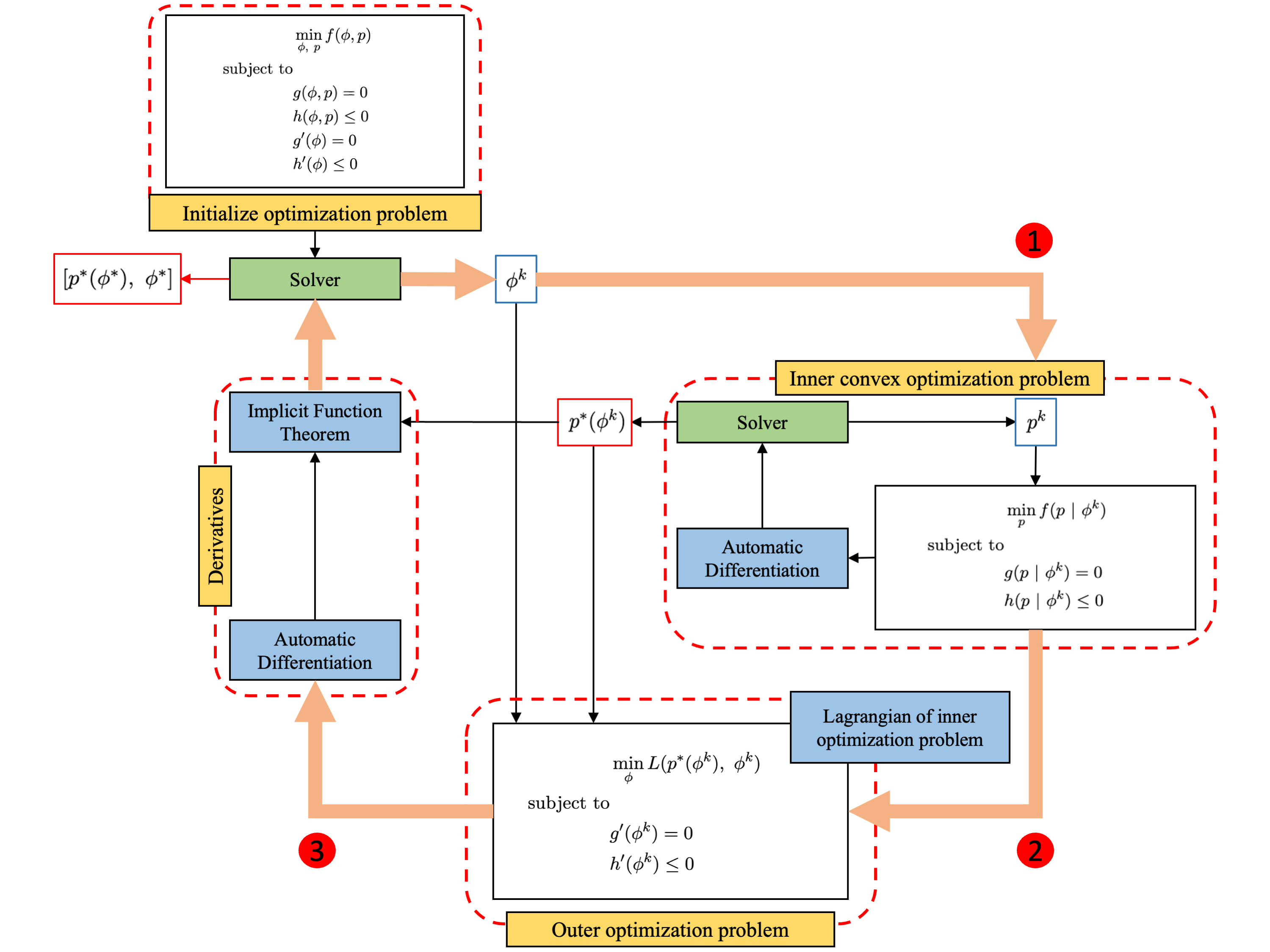
\[\begin{equation} p^{*} = \left [ \left ( \int _0^t f(\Psi(\hat{x}), p) \ dt \right) ^T \left ( \int _0^t f(\Psi(\hat{x}), p) \ dt \right ) \right ]^{-1} \left( \int_0^t f(\Psi(\hat{x}), p) \ dt \right) ^T (\hat{x}(t) - \hat{x}(t = 0)) \end{equation}\]This approach, however, is limited to cases where $p$ is linearly separable. The bilevel approach extends this idea to scenarios where $p$ may or may not be linearly separable. In such cases, we distinguish between parameters that appear linearly, denoted by $p$, and those that appear nonlinearly, denoted by $\phi$. We then formulate a bilevel optimization problem, where the inner problem solves a convex optimization over the linear parameters, while the outer problem optimizes the nonlinear parameters. Note that the inner optimization problem need not necessarily be convex; however, we observe that convexity in the inner problem leads to faster convergence. A schematic of the overall procedure is shown below.
We then modify the parameter estimation problem to account for linearly and nonlinearly separable parameters as follows
\[\begin{equation} \begin{aligned} \min _{p, \phi} f(p, \phi) = & \ \frac{1}{2} \sum_{t = t_i}^{t_f} || \hat{x}(t) - \hat{x}(0) - \int_0^t f(\Psi(\hat{x}), p, \phi) dt ||^2 \\ \text{subject to} & \\ & g(p, \phi) = 0 \\ & h(p, \phi) \leq 0 \\ & g'(\phi) = 0 \\ & h'(\phi) \leq 0 \end{aligned} \end{equation}\]where the equality constraints $g$ are affine in $p$ and the inequality constraints $h$ are convex in $p$. On the other hand, $g^{\prime}$ and $h^{\prime}$ can be any nonlinear equality and inequality constraints. Thus given the value of $\phi$, the above optimization problem becomes convex.
2.1 Derivatives of Inner Optimization Problem
Since we solve a bi-level optimization problem, we need to find the derivatives across the inner optimization problem. We form the Lagrangian of the inner convex optimization problem as follows
\[\begin{equation} \begin{aligned} L(p, \lambda, \mu \ | \ \phi) & = f(p | \phi) + \lambda ^T g(p | \phi) + \mu ^T h(p | \phi)\\ C(p^*, \lambda ^*, \mu ^*) & = \ \begin{cases} f_p(p^* | \phi) + \lambda ^*{}^T g_{p}(p^* | \phi) + \mu ^*{}^T h_p(p^* | \phi) = 0 \quad \text{Stationarity} \\[4pt] g(p^* | \phi) = 0 \quad \text{Primal feasibility} \\[4pt] \text{diag}(\mu ^*) h(p^* | \phi) = 0 \quad \text{complementary Slackness} \end{cases} \end{aligned} \end{equation}\]where $\lambda \in \mathbb{R}^{g}$ and $ \mu \in \mathbb{R}^{h}$ are the Lagrange variables of equality and inequality constraints, respectively. The optimal solution that satisfies the above equation is given as $(p^{\ast}(\phi), \lambda ^{\ast}, \mu ^{\ast})$. The derivative of the optimal solution with respect to $\phi$ can be efficiently calculated using the implicit function theorem 3. We derive equations used in forward-mode derivative calculations as follows
\[\begin{equation} \begin{aligned} \frac{d}{d \phi} C(p^* (\phi), \lambda ^* (\phi), \mu ^* (\phi)) & = 0 \\ \begin{bmatrix} \frac{dp ^*}{d \phi} \\[6pt] \frac{d\lambda ^*}{d\phi} \\[6pt] \frac{d \mu^*}{d \phi}\\[6pt] \end{bmatrix} v & = - \begin{bmatrix} L_{pp} & g_p^T & h_p^T\\[3pt] g_{p} & 0 & 0\\[3pt] \text{diag}(\mu) h_p & 0 & \text{diag}(h) \end{bmatrix} ^{-1} \begin{bmatrix} L_{p\phi} \\[3pt] g_{\phi} \\[3pt] \text{diag}(\mu ^*)h_{\phi} \end{bmatrix} v \end{aligned} \end{equation}\]where $v$ is the tangent vector used in forward-mode automatic differentiation. $(g_p, h_p)$ and $(g_{\phi}, h_{\phi})$ are the Jacobian of equality and inequality constraints with $p$ and $\phi$, respectively. $L_{pp}$ is the Hessian of the Lagrangian with respect to $p$. The factorization of the KKT matrix, or the Hessian of the Lagrangian at the optimal point, can be obtained from the optimization solver and reused in derivative calculations. We provide the necessary steps in case the factorization of the KKT matrix is unavailable.
\[\begin{equation} \begin{aligned} \begin{bmatrix} L_{pp} & g_p^T & h_p^T\\[3pt] g_{p} & 0 & 0\\[3pt] \text{diag}(\mu) h_p & 0 & \text{diag}(h) \end{bmatrix} \begin{bmatrix} w_1 \\[3pt] w_2 \\[3pt] w_3 \end{bmatrix} & = \begin{bmatrix} v_1 \\[3pt] v_2 \\[3pt] v_3 \end{bmatrix} = - \begin{bmatrix} L_{p\phi} v \\[3pt] g_{\phi} v \\[3pt] \text{diag}(\mu ^*)h_{\phi} v \end{bmatrix} \end{aligned} \end{equation}\]where $v = [v_1, v_2, v_3]^T$ is the Jacobian-vector product of the optimality conditions with the tangent vector $v$ and $w = [w_1, w_2, w_3]^T$ is a vector of appropriate dimensions.
\[\begin{equation} \begin{aligned} L_{pp} w_1 + g_p^T w_2 + h_p^T w_3 & = v_1 \\ g_p w_1 & = v_2 \\ w_3 & = [\text{diag}(h)]^{-1} \left[ v_3 - \text{diag}(\mu) h_p w_1 \right] \end{aligned} \end{equation}\]Let $H = \text{diag}(h)$ and $M = \text{diag}(\mu)$ then, substituting for $w_3^T$ gives
\[\begin{equation} \begin{aligned} \begin{bmatrix} L_{pp} - h_p^T M H^{-1} h_p & g_p^T \\[3pt] g_{p} & 0 \\ \end{bmatrix} \begin{bmatrix} w_1 \\[3pt] w_2 \\ \end{bmatrix} & = - \begin{bmatrix} v_1 - h_p^T H^{-1} v_3 \\[3pt] v_2 \end{bmatrix} \end{aligned} \end{equation}\]Let \(\hat{L}_{pp} = L_{pp} - h_p^T MH^{-1} h_p, \quad \text{and} \quad \hat{v}_1 = v_1 - h_p^T H^{-1}v_3\)
Note that for equality constraint optimization problem, we get \(\hat{L}_{pp} = L_{pp}, \text{and} \hat{v}_1 = v_1\)
We get the remaining vectors of $w$ as follows
\[\begin{equation} \begin{aligned} w_2 & = \left[ g_p^T \hat{L}_{pp}^{-1}g_p \right]^{-1} [- v_2 + g_p \hat{L}_{pp}^{-1} \hat{v}_1] \\ w_1 & = \hat{L}_{pp}^{-1} \left[ \hat{v}_1 - g_p^T w_2 \right] \end{aligned} \end{equation}\]Finally, we return the sensitivity vector $w$
2.2 Derivatives of Outer Opitmization Problem
We consider the Lagrangian of the inner optimization problem as the objective of the outer optimization problem. We also assume that at the optimal solution of the inner optimization problem, none of the inequality constraints are active $h(p^{\ast} \mid \phi) \neq 0$ and therefore $\mu ^{\ast} = 0$. These assumptions make the KKT point regular 4 and simplify the computation of the gradient and Hessian of the outer objective with respect to $\phi$, as shown below
\[\begin{equation} \begin{aligned} \text{Outer Objective} & = L(p^*(\phi), \phi) \\ \text{Gradient} & = \underbrace{\frac{\partial L}{\partial p^*}}_{= 0} \frac{dp^*}{d\phi} + \frac{\partial L}{\partial \phi} \\ \text{Hessian} & = \left(\frac{dp^*}{d\phi} \right)^T \frac{\partial ^2 L}{\partial {p^*}^2} \left( \frac{dp^*}{d\phi} \right) + \underbrace{\frac{\partial L}{\partial p^*}}_{= 0} \frac{d^2p^*}{d\phi^2} + \frac{\partial ^2 L}{\partial \phi^2} \end{aligned} \end{equation}\]Since we only require the gradient of $p^{\ast}$ with respect to $\phi$, its computation can be accelerate by storing the decomposition of the matrix \(\hat{L}_{pp} \ \text{and} \ g_p \hat{L}_{pp} g_p\) during the forward pass, and reusing them when computing derivatives either using forward-mode or reverse-mode automatic differentiation. However, storing this decomposition compromises the accuracy of any higher-order derivatives of $p^*$ with respect to $\phi$. Fortunately, this is acceptable in our case, as we do not need any higher-order derivatives as shown in Equation 11. An additional advantage of reusing this decomposition, particularly in JAX, is that it makes the forward-mode equations linear in the input tangent space 5. As a result, a custom forward rule is sufficient for both forward- and reverse-mode automatic differentiation. This enables faster Hessian computation using the forward-over-reverse approach, compared to reverse-over-reverse mode in case when the decomposition is not reused.
2.3 Derivatives of Ordinary Differential Equations
Computing derivative of $p^{\ast}$ with respect to $\phi$ also requires computing sensitivities across the differential equation solver. Using the forward-mode optimize-then-discretize differentiation approach gives
\[\begin{equation} \begin{aligned} \frac{dX}{dt} & = f(x, p^*(\phi), \phi) \\ \frac{d}{d\phi}\frac{dx}{dt} & = \frac{d}{d\phi} f(x, p^*(\phi), \phi) = \frac{\partial f}{\partial x} \frac{dx}{d\phi} + \frac{\partial f}{\partial p^*} \frac{dp^*}{d\phi} + \frac{\partial f}{\partial \phi} \\ \frac{dS}{dt} & = \frac{\partial f}{\partial x} S + \frac{\partial f}{\partial p^*} \frac{dp^*}{d\phi} + \frac{\partial f}{\partial \phi} \end{aligned} \end{equation}\]However, using interpolation makes the sensitivity calculations cheaper and relatively more stable by preventing sensitivities over unstable trajectories.
\[\begin{equation} \begin{aligned} \frac{dx}{dt} & = f(\Psi(\hat{x})(t), p^*(\phi), \phi) \\ \frac{d}{d\phi}\frac{dX}{dt} & = \frac{d}{d\phi} f(\Psi(\hat{x})(t), p^*(\phi), \phi) = \frac{\partial f}{\partial p^*} \frac{dp^*}{d\phi} + \frac{\partial f}{\partial \phi} \\ \frac{dS}{dt} & = \frac{\partial f}{\partial p^*} \frac{dp^*}{d\phi} + \frac{\partial f}{\partial \phi} \end{aligned} \end{equation}\]See this post for a tutorial on coding an implicit function theorem to compute derivatives across the optimization process in JAX.
3. Examples
We will look at two examples. In the first, all states are measured during parameter estimation, whereas in the second, only some of the states are observed. We start by importing necessary packages.
import jax
import jax.numpy as jnp
import jax.random as jrandom
jax.config.update("jax_enable_x64", True)
from jax.experimental.ode import odeint
from jax import flatten_util, tree_util

import matplotlib.pyplot as plt # plotting
from cyipopt import minimize_ipopt # ipopt optimizer
from scipy.interpolate import CubicSpline # interpolation

from utils import differentiable_optimization, odeint_diffrax # discussed in another tutorial
3.1 Parameter Estimation (Fully Observed States)
We use the oscillatory dynamics of calcium ion in the eukaryotic cells. The dynamics consist of four differential equations given as follows
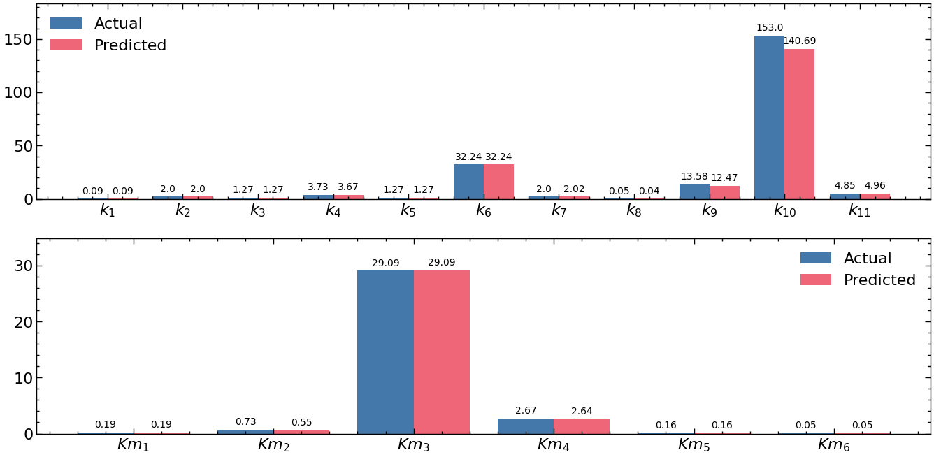
\[\begin{equation} \begin{aligned} \frac{dx_0}{dt} & = k_1 + k_2 x_0 - k_3 x_1 \frac{x_0}{x_0 + Km_1} - k_4 x_2 \frac{x_0}{x_0 + Km_2} \\ \frac{dx_1}{dt} & = k_5 x_0 - k_6 \frac{x_1}{x_1 + Km_3} \\ \frac{dx_2}{dt} & = k_7 x_1 x_2 \frac{x_3}{x_3 + Km_4} + k_8 x_1 + k_9 x_0 - k_{10} \frac{x_2}{x_2 + Km_5} - k_{11} \frac{x_2}{x_2 + Km_6} \\ \frac{dx_3}{dt} & = - k_7 x_1 x_2 \frac{x_3}{x_3 + Km_4} + k_{11} \frac{x_2}{x_2 + Km_6} \end{aligned} \end{equation}\]The linear parameters ($p$) are $k_1 = 0.09 $, $k_2 = 2 $, $k_3 = 1.27 $, $k_4 = 3.73 $, $k_5 = 1.27 $, $k_6 = 32.24 $, $k_7 = 2 $, $k_8 = 0.05 $, $k_9 = 13.58 $, $k_{10} = 153 $, $k_{11} = 4.85 $ and the nonlinear parameters ($\phi$) are $Km_1 = 0.19 $, $Km_2 = 0.73 $, $Km_3 = 29.09 $, $Km_4 = 2.67 $, $Km_5 = 0.16 $, $Km_6 = 0.05 $. The initial conditions are chosen to be $x_0(0) = 0.12 $, $x_1(0) = 0.31 $, $x_2(0) = 0.0058 $, $x_3(0) = 4.3 $. The model is simulated from $t_i = 0$ to $t_f = 60$(sec), and measurements are collected every $0.1$ seconds. For this set of parameters, the model exhibits a limit cycle. There are in total 17 parameters (11 appear linearly and 6 appear nonlinearly) to be estimated.
def calcium_ion(x, t, p) :
    (
        k1, k2, k3, k4, k5, k6,
        k7, k8, k9, k10, k11, km1,
        km2, km3, km4, km5, km6
    ) = p

    return jnp.array([
        k1 + k2 * x[0] - k3 * x[1] * x[0] / (x[0] + km1) - k4 * x[2] * x[0] / (x[0] + km2),
        k5 * x[0] - k6 * x[1] / (x[1] + km3),
        k7 * x[1] * x[2] * x[3] / (x[3] + km4) + k8 * x[1] + k9 * x[0] - k10 * x[2] / (x[2] + km5) - k11 * x[2] / (x[2] + km6),
        -k7 * x[1] * x[2] * x[3] / (x[3] + km4) + k11 * x[2] / (x[2] + km6)
    ])

# Generate data
nx = 4 # Number of states
key = jrandom.PRNGKey(20)
dt = 0.1 # measurement interval
xinit = jnp.array([0.12, 0.31, 0.0058, 4.3]) # Initial condition
time_span = jnp.arange(0, 20., dt) # Time span
p_actual = jnp.array([0.09, 2, 1.27, 3.73, 1.27, 32.24, 2, 0.05, 13.58, 153, 4.85, 0.19, 0.73, 29.09, 2.67, 0.16, 0.05]) # Actual parameters
solution = odeint(calcium_ion, xinit, time_span, p_actual) # Integrate
We use the cubic spline interpolation from scipy. This tutorial dicusses more on integrating a cubic spline interpolation in JAX.
class Interpolation():

    def __init__(self, solution, time_span):
        self.interpolations = CubicSpline(time_span, solution)

    def __call__(self, t):
        return self.interpolations(t)

class InterpolationDerivative():

    def __init__(self, interpolation : Interpolation, order : int = 1):
        self.derivatives = interpolation.interpolations.derivative(order)

    def __call__(self, t):
        return self.derivatives(t)


interpolations = Interpolation(solution, time_span)
interpolation_derivative = InterpolationDerivative(interpolations)

@jax.custom_jvp
def _interp(t) : return jax.pure_callback(interpolations, jax.ShapeDtypeStruct(xinit.shape, xinit.dtype), t)
_interp.defjvp(lambda primals, tangents : (_interp(*primals), None))

# Function that uses interpolation over states
def _foo_interp(z, t, px):
    p, x = px
    (
        k1, k2, k3, k4, k5, k6,
        k7, k8, k9, k10, k11
    ) = x

    (km1, km2, km3, km4, km5, km6) = p
    z = _interp(t)

    return jnp.array([
        k1 + k2 * z[0] - k3 * z[1] * z[0] / (z[0] + km1) - k4 * z[2] * z[0] / (z[0] + km2),
        k5 * z[0] - k6 * z[1] / (z[1] + km3),
        k7 * z[1] * z[2] * z[3] / (z[3] + km4) + k8 * z[1] + k9 * z[0] - k10 * z[2] / (z[2] + km5) - k11 * z[2] / (z[2] + km6),
        -k7 * z[1] * z[2] * z[3] / (z[3] + km4) + k11 * z[2] / (z[2] + km6)
    ])

# Inner objective function
def f(p, x, target):
    solution = odeint_diffrax(_foo_interp, xinit, time_span, (p.flatten(), x.flatten()), pargs.rtol, pargs.atol, pargs.mxstep) - xinit
    return jnp.mean((solution - target)**2)

# Equality constraints
def g(p, x) : return jnp.array([ ])

# Outer objective function
def simple_objective_shooting(f, g, p, states, target):
    (x_opt, v_opt), _ = differentiable_optimization(f, g, p, x_guess, (target, ))
    _loss = f(p, x_opt, target) + v_opt @ g(p, x_opt)
    return _loss, x_opt

# Outer optimization problem initialization
def outer_objective_shooting(p_guess, solution, target):

    # Create a temporary file to store optimization results
    _output_file = "ipopt_bilevelshootinginterp_output.txt"

    # JIT compiled objective function
    _simple_obj = jax.jit(lambda p : simple_objective_shooting(f, g, p, solution, target)[0])
    _simple_jac = jax.jit(jax.grad(_simple_obj))
    _simple_hess = jax.jit(jax.jacfwd(_simple_jac))

    def _simple_obj_error(p):
        try :
            sol = _simple_obj(p)
        except :
            sol = jnp.inf

        return sol

    solution_object = minimize_ipopt(
        _simple_obj_error,
        x0 = p_guess, # restart from intial guess
        jac = _simple_jac,
        hess = _simple_hess,
        tol = pargs.tol,
        options = {"maxiter" : pargs.iters, "output_file" : _output_file, "disp" : 0, "file_print_level" : 5, "mu_strategy" : "adaptive"}
        )

    # Once the optimization results are copied in our file, delete the temporary file
    shooting_logger.info(f"{divider}")
    with open(_output_file, "r") as file:
        for line in file : shooting_logger.info(line.strip())
    os.remove(_output_file)

    p = jnp.array(solution_object.x)
    loss, x = simple_objective_shooting(f, g, p, solution, target)
    return p, x.flatten()

dfsindy_target = solution - solution[0]
p, x = outer_objective_shooting(p_guess, solution, dfsindy_target)
******************************************************************************
This program contains Ipopt, a library for large-scale nonlinear optimization.
Ipopt is released as open source code under the Eclipse Public License (EPL).
For more information visit https://github.com/coin-or/Ipopt
******************************************************************************

This is Ipopt version 3.14.4, running with linear solver MUMPS 5.2.1.

Number of nonzeros in equality constraint Jacobian...:        0
Number of nonzeros in inequality constraint Jacobian.:        0
Number of nonzeros in Lagrangian Hessian.............:       21

Total number of variables............................:        6
variables with only lower bounds:        0
variables with lower and upper bounds:        0
variables with only upper bounds:        0
Total number of equality constraints.................:        0
Total number of inequality constraints...............:        0
inequality constraints with only lower bounds:        0
inequality constraints with lower and upper bounds:        0
inequality constraints with only upper bounds:        0

iter    objective    inf_pr   inf_du lg(mu)  ||d||  lg(rg) alpha_du alpha_pr  ls
0  3.2436101e+00 0.00e+00 1.23e+00   0.0 0.00e+00    -  0.00e+00 0.00e+00   0
1  2.4502986e+00 0.00e+00 8.11e-01 -11.0 6.54e-01   0.0 1.00e+00 1.00e+00f  1
2  2.1830382e+00 0.00e+00 7.02e-01 -11.0 2.59e-01   0.4 1.00e+00 1.00e+00f  1
Warning: Cutting back alpha due to evaluation error
3  1.8985871e+00 0.00e+00 6.08e-01 -11.0 5.59e-01  -0.1 1.00e+00 5.00e-01f  2
4  1.7541493e+00 0.00e+00 1.58e+01 -11.0 1.00e+00  -0.5 1.00e+00 1.00e+00f  1
5  9.5480522e-01 0.00e+00 2.39e+00 -11.0 1.44e+00  -1.0 1.00e+00 1.00e+00f  1
6  9.3503709e-01 0.00e+00 7.34e-01 -11.0 1.47e-02   1.2 1.00e+00 1.00e+00f  1
7  8.9229757e-01 0.00e+00 6.86e-01 -11.0 7.94e-02   0.7 1.00e+00 1.00e+00f  1
8  7.3584007e-01 0.00e+00 2.02e+00 -11.0 1.82e-01   1.2 1.00e+00 5.00e-01f  2
9  7.1222943e-01 0.00e+00 6.46e-01 -11.0 4.14e-02   0.7 1.00e+00 1.00e+00f  1
iter    objective    inf_pr   inf_du lg(mu)  ||d||  lg(rg) alpha_du alpha_pr  ls
10  6.8504690e-01 0.00e+00 1.98e-01 -11.0 1.19e-01   0.2 1.00e+00 1.00e+00f  1
11  6.2448297e-01 0.00e+00 1.77e-01 -11.0 3.16e-01  -0.3 1.00e+00 1.00e+00f  1
12  5.0958460e-01 0.00e+00 1.39e-01 -11.0 7.18e-01  -0.7 1.00e+00 1.00e+00f  1
13  3.5999822e-01 0.00e+00 9.27e-02 -11.0 1.30e+00  -1.2 1.00e+00 1.00e+00f  1
14  1.5810087e-01 0.00e+00 8.47e-02 -11.0 3.35e+00    -  1.00e+00 1.00e+00f  1
15  6.2181869e-02 0.00e+00 3.92e-02 -11.0 4.00e+00    -  1.00e+00 1.00e+00f  1
16  2.0850860e-02 0.00e+00 8.06e-03 -11.0 4.46e+00    -  1.00e+00 1.00e+00f  1
17  5.9221842e-03 0.00e+00 2.31e-02 -11.0 4.44e+00    -  1.00e+00 1.00e+00f  1
18  2.1207695e-03 0.00e+00 3.88e-02 -11.0 3.53e+00    -  1.00e+00 1.00e+00f  1
19  1.6713956e-03 0.00e+00 1.70e-01 -11.0 1.84e+00    -  1.00e+00 1.00e+00f  1
iter    objective    inf_pr   inf_du lg(mu)  ||d||  lg(rg) alpha_du alpha_pr  ls
20  1.6454504e-03 0.00e+00 1.11e-03 -11.0 3.93e-01    -  1.00e+00 1.00e+00f  1
21  1.6444131e-03 0.00e+00 3.50e-04 -11.0 1.20e-01    -  1.00e+00 1.00e+00f  1
22  1.6444069e-03 0.00e+00 1.20e-03 -11.0 1.37e-02    -  1.00e+00 1.00e+00f  1
23  1.6444057e-03 0.00e+00 5.22e-06 -11.0 8.46e-04    -  1.00e+00 1.00e+00f  1

Number of Iterations....: 23

(scaled)                 (unscaled)
Objective...............:   1.6444057248362022e-03    1.6444057248362022e-03
Dual infeasibility......:   5.2174389655213361e-06    5.2174389655213361e-06
Constraint violation....:   0.0000000000000000e+00    0.0000000000000000e+00
Variable bound violation:   0.0000000000000000e+00    0.0000000000000000e+00
Complementarity.........:   0.0000000000000000e+00    0.0000000000000000e+00
Overall NLP error.......:   5.2174389655213361e-06    5.2174389655213361e-06


Number of objective function evaluations             = 30
Number of objective gradient evaluations             = 24
Number of equality constraint evaluations            = 0
Number of inequality constraint evaluations          = 0
Number of equality constraint Jacobian evaluations   = 0
Number of inequality constraint Jacobian evaluations = 0
Number of Lagrangian Hessian evaluations             = 23
Total seconds in IPOPT                               = 2183.911

EXIT: Optimal Solution Found.
----------------------------------------------------------------------------------------------------
Loss 0.0016444082936688555
----------------------------------------------------------------------------------------------------
Nonlinear parameters : [ 0.18820301  0.55304131 29.09177972  2.63659125  0.16198204  0.05250169]
----------------------------------------------------------------------------------------------------
Linear parameters : [8.81149634e-02 2.00281068e+00 1.27131557e+00 3.66662276e+00
 1.27005579e+00 3.22425872e+01 2.02186745e+00 3.72664189e-02
 1.24711028e+01 1.40687511e+02 4.95685686e+00]
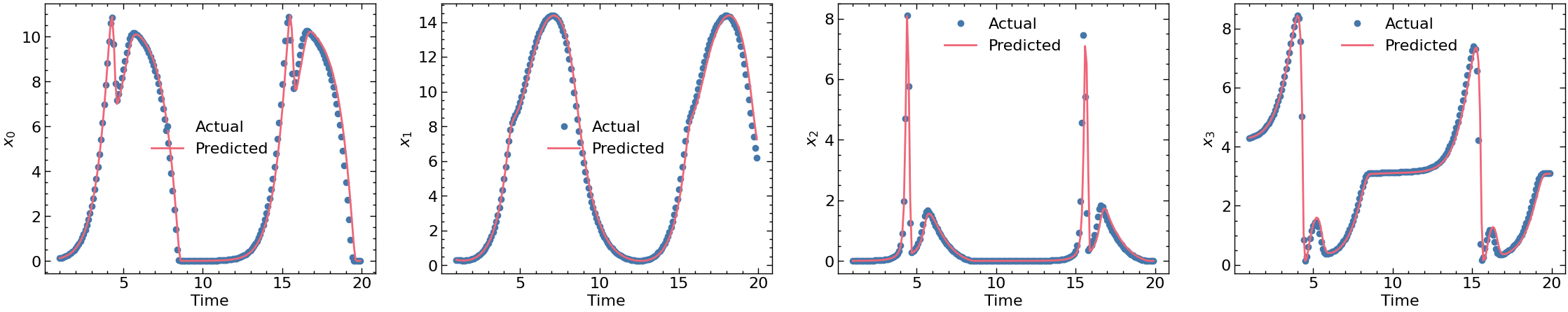
If we were to compare the estimated coefficients and their trajectories with original coefficients and their trajectories, we get the following plots
3.2 Parameter Estimation (Partially Observed States)
We use the dynamics of a continuously stirred tank reactor. The dynamics consist of four differential equations given as follows
\[\begin{equation} \begin{aligned} \frac{dx_0}{dt} & = -\beta (t) x_0 + F_{in} ( C_{in} - x_0) \\ \frac{dx_1}{dt} & = 130 * \beta (t) x_0 + F_{in} (T_{in} - x_1) + U (T_c - x_1) \\ \beta (t) & = k_{ref} e^{- EdivR 10^4 \left( \frac{1}{x_1} - \frac{1}{T_{ref}} \right)} \\ \end{aligned} \end{equation}\]where $x_0$ and $x_1$ are the concentration and temperature inside the reactor, $F_{in} = 1 $, $T_{in} = 323 $, and $C_{in} = 2 $ are the inlet flow rate, temperature and concentration of inlet stream. $T_c = 340 $ is the inlet temperature of the coolant used to control the temperature of the reactor, $U$ is the heat transfer coefficient, and $\beta $ is the reaction rate constant. The initial conditions are $x_0 (0) = 1.6 $ and $x_1 (0) = 340 $, which are know however only $x_1$ is measured and $x_0$ is not. Given the measurements of $x_1$ for $t_i = 0$ to $t_f = 10$(sec), and $ \Delta t = 0.1 $, we want to estimate the parameters of the model $k_{ref} = 0.461 $, $U = 5.3417 $, and $ EdivR = 0.833 $. Note that we assume that the system is identifiable with the current setting.
The idea is to treat the optimization problem corresponding to the unobserved states as a single-shooting problem (more in this tutorial), in which all the parameters (irrespective of whether they appear linearly or not) are treated as nonlinear, while the observed states are handled in the same way as in the previous example. Consequently there 2 nonlienar parameters and 1 linear parameters. Note that Another approach, often referred to as the cascading approach to parameter estimation, involves approximating the trajectory of the unobserved state (treated here as decision variables) using an interpolation function such as a cubic spline, as demonstrated previously. However, unlike before, these parameters are no longer fixed; they now depend on the unobserved state trajectory and therefore change with each iteration of the parameter estimation process. The remainder of the problem is treated in the same way. This approach requires a differentiable cubic spline interpolation function, which is provided in this tutorial. Although feasible, it tends to be computationally expensive, because of computing the Hessian with respect to all the additional interpolation parameters.
def cstr(x, t, p):
    Fin = 1 # Inflow
    Cin = 2 # Concentration of inflow
    Tin = 323 # Temperature of inflow
    Tc = 340 # Inlet temperature of coolant
    kref, U, EdivR = p # [0.461, 5.3417, 0.833]
    b = kref * jnp.exp(- 10**4 * EdivR * (1 / x[1] - 1 / 350))
    return jnp.array([
        - b * x[0] + Fin * (Cin - x[0]),
        130 * b * x[0] + Fin * (Tin - x[1]) + U * (Tc - x[1])
    ])

xinit = jnp.array([1.6, 340])
p_actual = jnp.array([0.461, 5.3417, 0.833])
time_span = jnp.arange(0, 10, 0.1)
solution = odeint_diffrax(cstr, xinit, time_span, p_actual)
We then define the objective function of the inner and outer optimization problems
def f(p, x, states, target):

    def cstr_interp(x, t, p):
        Fin = 1 # Inflow
        Cin = 2 # Concentration of inflow
        Tin = 323 # Temperature of inflow
        Tc = 340 # Temperature of coolant
        (kref, EdivR), (U, ) = p

        z = _interp(t)
        b = kref * jnp.exp(- 10**4 * EdivR * (1 / z[1] - 1 / 350))
        return jnp.array([
            - b * x[0] + Fin * (Cin - x[0]),
            130 * b * x[0] + Fin * (Tin - z[1]) + U * (Tc - z[1])
        ])

    solution = odeint_diffrax(cstr_interp, xinit, time_span, (p.flatten(), x.flatten())) - xinit
    return jnp.mean((solution[:, 1] - target)**2) # minimize over the temperature values only

def g(p, x) : return jnp.array([ ])

def simple_objective_shooting(f, g, p, states, target):
    (x_opt, v_opt), _ = differentiable_optimization(f, g, p, x_guess, (states, target))
    _loss = f(p, x_opt, states, target) + v_opt @ g(p, x_opt)
    return _loss, x_opt

def outer_objective_shooting(p_guess, states, target):

    _output_file = "ipopt_bilevelshootinginterp_output.txt"

    # JIT compiled objective function
    _simple_obj = jax.jit(lambda p : simple_objective_shooting(f, g, p, states, target)[0])
    _simple_jac = jax.jit(jax.grad(_simple_obj))
    _simple_hess = jax.jit(jax.jacfwd(_simple_jac))

    def _simple_obj_error(p):
        try :
            sol = _simple_obj(p)
        except :
            sol = jnp.inf

        return sol

    solution_object = minimize_ipopt(
        _simple_obj_error,
        x0 = p_guess, # restart from intial guess
        jac = _simple_jac,
        hess = _simple_hess,
        tol = 1e-5,
        options = {"maxiter" : 1000, "output_file" : _output_file, "disp" : 0, "file_print_level" : 5, "mu_strategy" : "adaptive"}
        )

    shooting_logger.info(f"{divider}")
    with open(_output_file, "r") as file:
        for line in file : shooting_logger.info(line.strip())
    os.remove(_output_file)

    p = jnp.array(solution_object.x)
    return p, x.flatten()
******************************************************************************
This program contains Ipopt, a library for large-scale nonlinear optimization.
Ipopt is released as open source code under the Eclipse Public License (EPL).
For more information visit https://github.com/coin-or/Ipopt
******************************************************************************

This is Ipopt version 3.14.4, running with linear solver MUMPS 5.2.1.

Number of nonzeros in equality constraint Jacobian...:        0
Number of nonzeros in inequality constraint Jacobian.:        0
Number of nonzeros in Lagrangian Hessian.............:        3

Total number of variables............................:        2
variables with only lower bounds:        0
variables with lower and upper bounds:        0
variables with only upper bounds:        0
Total number of equality constraints.................:        0
Total number of inequality constraints...............:        0
inequality constraints with only lower bounds:        0
inequality constraints with lower and upper bounds:        0
inequality constraints with only upper bounds:        0

iter    objective    inf_pr   inf_du lg(mu)  ||d||  lg(rg) alpha_du alpha_pr  ls
0  1.7280182e+02 0.00e+00 1.00e+02   0.0 0.00e+00    -  0.00e+00 0.00e+00   0
1  2.2261013e+01 0.00e+00 2.55e+01 -11.0 7.52e-01    -  1.00e+00 1.00e+00f  1
2  1.1322034e+00 0.00e+00 4.68e+00 -11.0 2.47e-01   2.0 1.00e+00 1.00e+00f  1
3  1.4371045e-02 0.00e+00 6.76e-01 -11.0 1.48e-01    -  1.00e+00 1.00e+00f  1
4  3.5321911e-06 0.00e+00 8.73e-03 -11.0 1.52e-02    -  1.00e+00 1.00e+00f  1
5  6.9815428e-09 0.00e+00 2.50e-06 -11.0 2.78e-04    -  1.00e+00 1.00e+00f  1

Number of Iterations....: 5

(scaled)                 (unscaled)
Objective...............:   1.1939052466347747e-09    6.9815427997590546e-09
Dual infeasibility......:   2.5035343383026149e-06    1.4639798411802267e-05
Constraint violation....:   0.0000000000000000e+00    0.0000000000000000e+00
Variable bound violation:   0.0000000000000000e+00    0.0000000000000000e+00
Complementarity.........:   0.0000000000000000e+00    0.0000000000000000e+00
Overall NLP error.......:   2.5035343383026149e-06    1.4639798411802267e-05


Number of objective function evaluations             = 6
Number of objective gradient evaluations             = 6
Number of equality constraint evaluations            = 0
Number of inequality constraint evaluations          = 0
Number of equality constraint Jacobian evaluations   = 0
Number of inequality constraint Jacobian evaluations = 0
Number of Lagrangian Hessian evaluations             = 5
Total seconds in IPOPT                               = 144.920

EXIT: Optimal Solution Found.
----------------------------------------------------------------------------------------------------
Loss 6.981542799759055e-09
----------------------------------------------------------------------------------------------------
Nonlinear parameters : [0.46098732 0.83299782]
----------------------------------------------------------------------------------------------------
Linear parameters : [5.34155304]
4. Conclusion
We saw how a bilevel optimization, coupled with interpolation, can be used to perform parameter etimation. Because of using interpolation, this approach exploits the convexity of some parameters that appear linearly in the dynamic equation. We then test this method on both fully observed and partially observed parameter estimation problems
5. References
-
Siddharth Prabhu, Srinivas Rangarajan, and Mayuresh Kothare. Bi-level optimization for parameter estimation of differential equations using interpolation, 2025. ↩
-
Siddharth Prabhu, Nick Kosir, Mayuresh Kothare, and Srinivas Rangarajan. Derivative-free domain-informed data-driven discovery of sparse kinetic models. Industrial & Engineering Chemistry Research, 2025 ↩
-
Steven George Krantz and Harold R Parks. The implicit function theorem: history, theory, and applications. Springer Science & Business Media, 2002. ↩
-
Diehl, M., Gros, S., 2011. Numerical optimal control. Optimization in Engineering Center (OPTEC) ↩
-
James Bradbury, Roy Frostig, Peter Hawkins, Matthew James Johnson, Chris Leary, Dougal Maclaurin, George Necula, Adam Paszke, Jake VanderPlas, Skye Wanderman-Milne, and Qiao Zhang. JAX: composable transformations of Python+NumPy programs, 2018. ↩